Free vibration of a clamped square plate

This example computes the natural frequencies and mode shapes of a square plate clamped along its entire boundary. A modal analysis solves the generalized eigenvalue problem

\[\mathbf{K}\boldsymbol{\phi} = \omega^2 \mathbf{M}\boldsymbol{\phi},\]

where \(\mathbf{K}\) and \(\mathbf{M}\) are the stiffness and mass matrices, \(\omega\) is an angular frequency, and \(\boldsymbol{\phi}\) is a mode shape. Because no external load is needed, this analysis is also called a free-vibration analysis.

import numpy as np
import pyvista as pv

import fedoo as fd

Geometry and mesh

The one-metre square mid-surface is discretized with quadrilateral shell elements. Its thickness is small compared with its in-plane dimensions.

fd.ModelingSpace("3D")

length = 1.0
thickness = 0.01
mesh = fd.mesh.rectangle_mesh(
    nx=15,
    ny=15,
    x_min=0.0,
    x_max=length,
    y_min=0.0,
    y_max=length,
    elm_type="quad4",
    ndim=3,
)

Material, shell section, and assembly

ShellHomogeneous integrates the elastic material through the specified thickness. The material density supplies the translational and rotary inertia used to assemble the shell mass matrix.

steel = fd.constitutivelaw.ElasticIsotrop(210e9, 0.3)
steel.set_density(7800.0)
shell = fd.constitutivelaw.ShellHomogeneous(steel, thickness)
weakform = fd.weakform.PlateEquilibrium(shell)
assembly = fd.Assembly.create(weakform, mesh)

Modal problem

A clamped shell boundary has zero translations and zero rotations. The four edge node sets are combined so that this condition is applied around the complete perimeter. sigma=0 asks the sparse eigensolver for the four modes closest to zero frequency.

Registering an output writes one frame per mode to the fdh5 file. Each frame also contains the mode number, eigenvalue, angular frequency, and frequency as scalar metadata.

boundary = np.unique(
    np.concatenate(
        [mesh.node_sets[name] for name in ("left", "right", "bottom", "top")]
    )
)

modal = fd.problem.Modal(assembly)
modal.bc.add("Dirichlet", boundary, ["Disp", "Rot"], 0.0)
results = modal.add_output(
    "clamped_plate_modes.fdh5",
    assembly,
    ["Disp", "Rot", "Strain", "Stress"],
)
modal.solve(n_modes=4, sigma=0.0)

print("Natural frequencies [Hz]:")
for mode, frequency in enumerate(modal.frequencies, start=1):
    print(f"  mode {mode}: {frequency:.6g}")

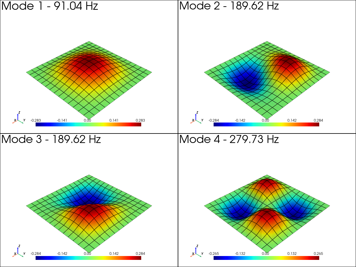
Natural frequencies [Hz]:
  mode 1: 91.041
  mode 2: 189.619
  mode 3: 189.619
  mode 4: 279.734

Plot the first four mode shapes

Eigenvectors have no physical amplitude. Each mode is therefore scaled so that its maximum transverse displacement is 15% of the plate width. The four saved frames are drawn in a shared 2-by-2 PyVista plotter through the standard fedoo.DataSet plotting interface. multiplot=True gives every subplot its own mesh actor and scalar bar.

plotter = pv.Plotter(shape=(2, 2), window_size=(1200, 900))
for mode_index, frequency in enumerate(modal.frequencies):
    results.load(mode_index)
    transverse_displacement = results["Disp"][2]
    amplitude = np.max(np.abs(transverse_displacement))
    display_scale = 0.15 * length / amplitude

    plotter.subplot(*divmod(mode_index, 2))
    results.plot(
        "Disp",
        component="Z",
        iteration=mode_index,
        scale=display_scale,
        clim=[-amplitude, amplitude],
        plotter=plotter,
        show=False,
        show_edges=True,
        multiplot=True,
        title=f"Mode {mode_index + 1} - {frequency:.2f} Hz",
    )

plotter.link_views()
plotter.view_isometric()
plotter.show()