Visualization tutoral - Shear test of a cube

This example performs a displacement-driven shear test on a unit cube using a finite-strain formulation. Several post-processing and visualization options are demonstrated, including:

• Scalar field visualization (von Mises stress)

• Side-by-side linked views

• Clipping with a plane

• Element-set filtering from arbitrary expressions

• Sampling and plotting results along a line

• Plotting the time evoluation of a field value.

import fedoo as fd
import numpy as np
import pyvista as pv
import matplotlib.pyplot as plt

fd.get_config()["USE_PYVISTA_QT"] = False  # avoid rendering useless plot

Geometry and mesh

A regular hexahedral mesh of a unit cube is generated.

fd.ModelingSpace("3D")

# Hexahedral regular mesh of an unit cube
mesh = fd.mesh.box_mesh(
    nx=11,
    ny=11,
    nz=11,  # adjust for finer/coarser runs
    x_min=0,
    x_max=1,
    y_min=0,
    y_max=1,
    elm_type="hex8",
)

Constitutive law and weak form

Elasto-plastic constitutive law with power-law hardening, solved using a finite-strain formulation.

props = np.array(
    [
        200e3,  # Young modulus [MPa]
        0.3,  # Poisson ratio
        1e-5,  # thermal expansion coefficient (unused here)
        300.0,  # yield stress
        1000.0,  # hardening coefficient
        0.3,  # hardening exponent
    ]
)

material = fd.constitutivelaw.Simcoon("EPICP", props)
wf = fd.weakform.StressEquilibriumRI(material, nlgeom="UL")

assembly = fd.Assembly.create(wf, mesh)

Problem definition

Nonlinear static problem with displacement-controlled loading.

pb = fd.problem.NonLinear(assembly)

results = pb.add_output(
    "shear.fdz",
    assembly,
    ["Disp", "Stress", "Strain", "P", "Fext"],
)

Boundary conditions

The bottom face is fixed. A horizontal displacement is imposed on the top face to create shear.

nodes_bottom = mesh.find_nodes("Y", 0.0)
nodes_top = mesh.find_nodes("Y", 1.0)

pb.bc.add("Dirichlet", nodes_bottom, "Disp", 0.0)
pb.bc.add("Dirichlet", nodes_top, ["DispY", "DispZ"], [0.0, 0.0])
pb.bc.add("Dirichlet", nodes_top, "DispX", -0.5)

Dirichlet boundary condition:
var = 'DispX'
n_nodes = 121
value = -0.5

Solve the problem

pb.nlsolve(dt=0.05, tmax=1.0, update_dt=True, interval_output=0.05, print_info=0)

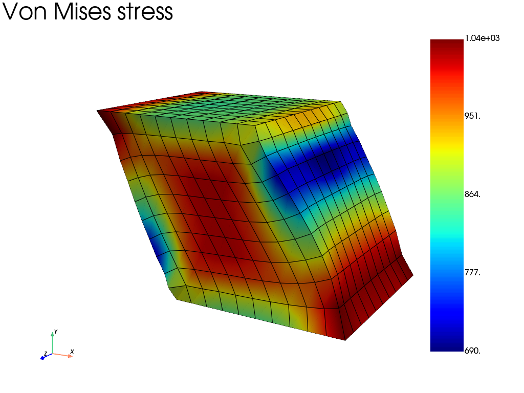
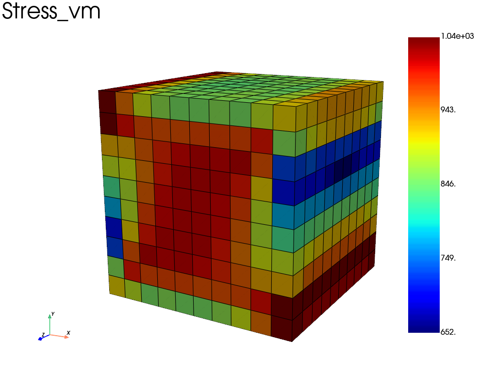
Basic visualization: von Mises stress

Plot the von Mises stress on the deformed mesh.

res_plot = results.plot(
    field="Stress",
    component="vm",
    data_type="Node",
    show_edges=True,
    title="Von Mises stress",
)

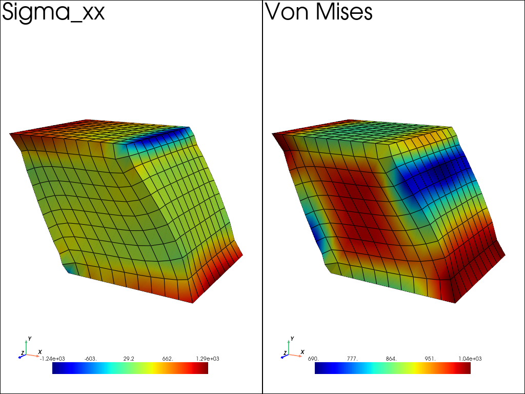
Side-by-side linked views

Compare σ_xx and von Mises stress using linked cameras.

pl = pv.Plotter(shape=(1, 2))

pl.subplot(0, 0)
results.plot(
    "Stress",
    "XX",
    "Node",
    plotter=pl,
    show=False,
    multiplot=True,
    title="Sigma_xx",
)
pl.camera.view_angle = 40.0

pl.subplot(0, 1)
results.plot(
    "Stress",
    "vm",
    "Node",
    plotter=pl,
    show=False,
    multiplot=True,
    title="Von Mises",
)
pl.link_views()  # use same view angle for both subplots
pl.show()

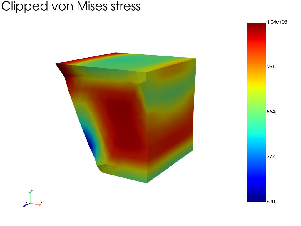
Clipping with a plane

Clip the mesh using a plane normal to the X direction.

clip_args = dict(
    normal=(1.0, 0.0, 0.0),
    origin=(0.5, 0.5, 0.5),
)

pl = results.plot(
    "Stress",
    "vm",
    "Node",
    clip_args=clip_args,
    show_edges=False,
    title="Clipped von Mises stress",
)

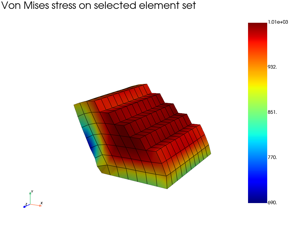
Element-set filtering from an expression

Select elements inside a cylindrical region defined by X² + Y² < 0.25. The element selection is based on element center coordinates.

element_ids = mesh.find_elements("X**2 + Y**2 < 0.5")

pl = results.plot(
    "Stress",
    "vm",
    "Node",
    element_set=element_ids,
    title="Von Mises stress on selected element set",
)

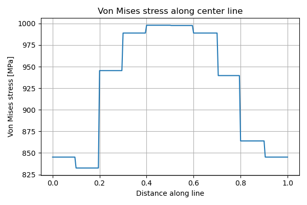
Sampling results along a line

Extract the von Mises stress along a line passing through the cube center.

pl = results.plot(
    "Stress",
    "vm",
    # "Node",  # uncomment to avarage results at nodes
    scale=0,
    show=False,  # just used to build the mesh here
)
pv_mesh = pl.actors["data1"].mapper.dataset  # extract the mesh

profile = pv_mesh.sample_over_line(
    (0.0, 0.5, 0.5),
    (1.0, 0.5, 0.5),
    resolution=200,
)

distance_key = "Distance" if "Distance" in profile.point_data else "arc_length"
vm_key = profile.active_scalars_name

plt.figure(figsize=(6, 4))
plt.plot(profile.point_data[distance_key], profile.point_data[vm_key])
plt.xlabel("Distance along line")
plt.ylabel("Von Mises stress [MPa]")
plt.title("Von Mises stress along center line")
plt.grid(True)
plt.tight_layout()
plt.show()

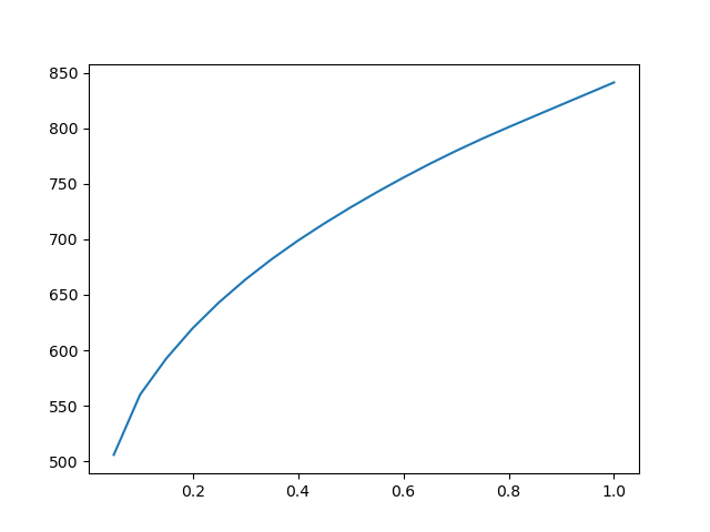
History plot at selected nodes

When results are written at multiple time steps, the result object is a MultiFrameDataSet. History plots can be generated directly using the plot_history method.

# Select a node at the center of the top face
center_node = mesh.nearest_node([0.5, 1, 0.5])

# Plot the von Mises stress history at this node
results.plot_history(
    field="Stress",
    indices=center_node,
    component="vm",
    data_type="Node",
)