Stress transfer: Cauchy → PKI/PKII/Kirchhoff

This example is an hands-on demo of the stress “transfer” helpers in simcoon.simmit to switch between different stress measures.

We compute the Cauchy stress for a compressible Neo-Hookean material, then use simcoon.simmit.stress_convert() to obtain other stress measures:

• First Piola-Kirchhoff stress (PKI)

• Second Piola-Kirchhoff stress (PKII)

• Kirchhoff stress

To get a physically meaningful uniaxial response, the lateral stretch is solved so that transverse Cauchy stresses are (approximately) zero (free contraction), similar to the uniaxial tension path used in the hyperelastic numerical example.

The focus is on data shape conventions and on using the batch conversion API. Throughout the script we use the batch layouts expected by the bindings:

• stress batches as (6, N)

• deformation-gradient batches as (3, 3, N)

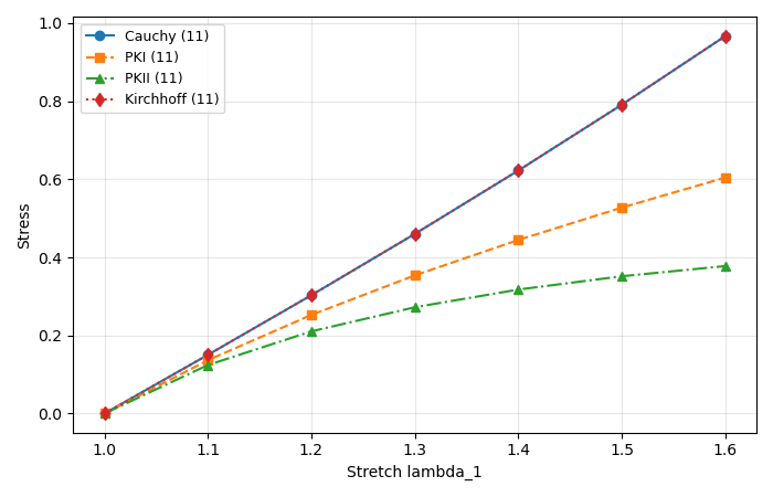
At the end we plot only the 11 component (Voigt index 0) for a quick comparison between stress measures.

from __future__ import annotations

import numpy as np
from simcoon import simmit as sim
import matplotlib.pyplot as plt
from scipy.optimize import fsolve

Helpers

We implement two tiny helpers:

• a Neo-Hookean Cauchy stress evaluator using the invariants-based API

• a “free contraction” uniaxial deformation gradient F = diag(lam1, lt, lt) where lt is solved such that the transverse stresses are ~0.

def neo_hookean_cauchy(F: np.ndarray, mu: float, kappa: float) -> np.ndarray:
    """Return Cauchy stress for a compressible Neo-Hookean (invariants form).

    Inputs
    - F: (3,3) deformation gradient
    - mu, kappa: shear modulus and bulk modulus
    """

    J = float(np.linalg.det(F))
    b = sim.L_Cauchy_Green(F)

    # Neo-Hookean: W_iso = mu/2 * (I1_bar - 3), U(J) = kappa/2 (ln J)^2
    dWdI_1_bar = 0.5 * float(mu)
    dWdI_2_bar = 0.0
    dUdJ = float(kappa) * np.log(J)

    sigma_iso = sim.sigma_iso_hyper_invariants(dWdI_1_bar, dWdI_2_bar, b, J, False)
    sigma_vol = sim.sigma_vol_hyper(dUdJ, b, J, False)
    return np.asarray(sigma_iso + sigma_vol, dtype=float)


def free_contraction_F(
    lam1: float, mu: float, kappa: float, lt_guess: float
) -> tuple[np.ndarray, float]:
    """Uniaxial tension with free lateral contraction.

    Solve lt such that sigma_22 = sigma_33 = 0 for F = diag(lam1, lt, lt).
    Returns (F, lt).
    """

    def equilibrium(lt_arr: np.ndarray) -> float:
        lt = float(lt_arr[0])
        F = np.diag([float(lam1), lt, lt])
        sigma = neo_hookean_cauchy(F, mu=mu, kappa=kappa)
        # symmetric lateral directions: drive the average transverse stress to zero
        return float(0.5 * (sigma[1, 1] + sigma[2, 2]))

    lt = float(fsolve(equilibrium, np.array([lt_guess]))[0])
    F = np.diag([float(lam1), lt, lt])
    return F, lt

Uniaxial stretch sweep (free contraction)

We sweep the axial stretch lambda_1 and solve the lateral stretch lambda_t at each point (using the previous lambda_t as initial guess).

Data is stored directly into batch arrays:

• sigma_cauchy_batch has shape (6, N)

• F_batch has shape (3, 3, N)

# Simple Neo-Hookean parameters
mu = 0.5
kappa = 1000.0

lam1_vals = np.linspace(1.0, 1.6, 7)

# We keep batch arrays from the get-go:
#   sigma_*_batch: (6, N)
#   F_batch: (3, 3, N)
N = int(lam1_vals.size)
sigma_cauchy_batch = np.zeros((6, N), dtype=float)
F_batch = np.zeros((3, 3, N), dtype=float)
lt_vals = np.zeros((N,), dtype=float)

lt_guess = 1.0

for i, lam1 in enumerate(lam1_vals):
    F, lt = free_contraction_F(float(lam1), mu=mu, kappa=kappa, lt_guess=lt_guess)
    lt_guess = lt
    F_batch[:, :, i] = F
    lt_vals[i] = lt

    sigma = neo_hookean_cauchy(F, mu=mu, kappa=kappa)
    sigma_v = np.asarray(sim.t2v_stress(sigma), dtype=float).reshape(6)
    sigma_cauchy_batch[:, i] = sigma_v

# Convert Cauchy -> PK1 and Cauchy -> PK2 for comparison
sigma_pk1_batch = sim.stress_convert(sigma_cauchy_batch, F_batch, "Cauchy2PKI")
sigma_pk2_batch = sim.stress_convert(sigma_cauchy_batch, F_batch, "Cauchy2PKII")
sigma_kirchhoff_batch = sim.stress_convert(
    sigma_cauchy_batch, F_batch, "Cauchy2Kirchhoff"
)

Post-processing: quick comparison between stress measures

Conversions (same physical state, different stress measures):

• Kirchhoff stress: \(\boldsymbol{\tau} = J\,\boldsymbol{\sigma}\)

• First Piola–Kirchhoff (PKI): \(\mathbf{P} = J\,\boldsymbol{\sigma}\,\mathbf{F}^{-T}\)

• Second Piola–Kirchhoff (PKII): \(\mathbf{S} = \mathbf{F}^{-1}\mathbf{P} = J\,\mathbf{F}^{-1}\boldsymbol{\sigma}\,\mathbf{F}^{-T}\)

where \(\boldsymbol{\sigma}\) is the Cauchy stress, \(\mathbf{F}\) is the deformation gradient, and \(J = \det(\mathbf{F})\).

In this demo, the “free contraction” solution with a large bulk modulus (nearly incompressible response) keeps \(J \approx 1\), so \(\boldsymbol{\tau}\) and \(\boldsymbol{\sigma}\) nearly overlap (up to the factor \(J\). We print a simple \(J\) diagnostic below.

J_vals = np.linalg.det(np.transpose(F_batch, (2, 0, 1)))  # (N,)
print(f"J deviation: min(J)={J_vals.min():.6f}, max(J)={J_vals.max():.6f}")

# For printing/plotting it's convenient to view as (N,6)
sigma_cauchy = sigma_cauchy_batch.T
sigma_pk1 = np.asarray(sigma_pk1_batch, dtype=float).T
sigma_pk2 = np.asarray(sigma_pk2_batch, dtype=float).T
sigma_kirchhoff = np.asarray(sigma_kirchhoff_batch, dtype=float).T

# Print one snapshot (so the example still shows raw numbers)
i_show = int(len(lam1_vals) // 2)
F_show = F_batch[:, :, i_show]
sig_show = sim.v2t_stress(np.ascontiguousarray(sigma_cauchy_batch[:, i_show]))
print("Uniaxial stretch demo")
print("--------------------")
print(f"mu={mu}, kappa={kappa}")
print(f"lambda_1 = {lam1_vals[i_show]:.3f}")
print(f"lambda_t = {lt_vals[i_show]:.6f}")
print("F =")
print(F_show)
print("Cauchy stress (3x3) =")
print(sig_show)

# Plot the 11-component for several stress measures
# Voigt order is assumed [11, 22, 33, 12, 23, 13] (simcoon convention).
comp_11 = 0

fig, ax = plt.subplots(figsize=(7.0, 4.5))
ax.plot(lam1_vals, sigma_cauchy[:, comp_11], "-o", label="Cauchy (11)")
ax.plot(lam1_vals, sigma_pk1[:, comp_11], "--s", label="PKI (11)")
ax.plot(lam1_vals, sigma_pk2[:, comp_11], "-.^", label="PKII (11)")
ax.plot(lam1_vals, sigma_kirchhoff[:, comp_11], ":d", label="Kirchhoff (11)")

ax.set_xlabel("Stretch lambda_1")
ax.set_ylabel("Stress")
ax.grid(True, alpha=0.3)
ax.legend(fontsize=9)
fig.tight_layout()
plt.show()

J deviation: min(J)=1.000000, max(J)=1.000322
Uniaxial stretch demo
--------------------
mu=0.5, kappa=1000.0
lambda_1 = 1.300
lambda_t = 0.877125
F =
[[1.3        0.         0.        ]
 [0.         0.87712529 0.        ]
 [0.         0.         0.87712529]]
Cauchy stress (3x3) =
[[ 4.60207933e-01  0.00000000e+00  0.00000000e+00]
 [ 0.00000000e+00 -1.14912191e-10  0.00000000e+00]
 [ 0.00000000e+00  0.00000000e+00 -1.14912191e-10]]