Transversely Isotropic Elasticity Example

import numpy as np
from simcoon import simmit as sim
import matplotlib.pyplot as plt
import os

In transversely isotropic elastic materials, there is a single axis of symmetry. The material behaves isotropically in the plane perpendicular to this axis (the transverse plane). Eight parameters are required:

1. The axis of symmetry (1, 2, or 3)

2. The longitudinal Young modulus \(E_L\)

3. The transverse Young modulus \(E_T\)

4. The Poisson ratio in the transverse-longitudinal plane \(\nu_{TL}\)

5. The Poisson ratio in the transverse-transverse plane \(\nu_{TT}\)

6. The shear modulus in the longitudinal-transverse plane \(G_{LT}\)

7. The coefficient of thermal expansion in the longitudinal direction \(\alpha_L\)

8. The coefficient of thermal expansion in the transverse direction \(\alpha_T\)

The elastic stiffness tensor for a transversely isotropic material with axis 1 as the symmetry axis is written in the Voigt notation formalism as:

\[\begin{split}\mathbf{L} = \begin{pmatrix} L_{11} & L_{12} & L_{12} & 0 & 0 & 0 \\ L_{12} & L_{22} & L_{23} & 0 & 0 & 0 \\ L_{12} & L_{23} & L_{22} & 0 & 0 & 0 \\ 0 & 0 & 0 & G_{TT} & 0 & 0 \\ 0 & 0 & 0 & 0 & G_{LT} & 0 \\ 0 & 0 & 0 & 0 & 0 & G_{LT} \end{pmatrix}\end{split}\]

where \(G_{TT} = E_T / (2(1+\nu_{TT}))\) is the shear modulus in the transverse plane.

The thermal expansion tensor is:

\[\begin{split}\boldsymbol{\alpha} = \begin{pmatrix} \alpha_L & 0 & 0 \\ 0 & \alpha_T & 0 \\ 0 & 0 & \alpha_T \end{pmatrix}\end{split}\]

umat_name = "ELIST"  # 5 character code for transversely isotropic elastic subroutine
nstatev = 1  # Number of internal variables

# Material parameters
axis = 1  # Symmetry axis
E_L = 4500.0  # Longitudinal Young's modulus (MPa)
E_T = 2300.0  # Transverse Young's modulus (MPa)
nu_TL = 0.05  # Poisson ratio (transverse-longitudinal)
nu_TT = 0.3  # Poisson ratio (transverse-transverse)
G_LT = 2700.0  # Shear modulus (longitudinal-transverse)
alpha_L = 1.0e-5  # Thermal expansion (longitudinal)
alpha_T = 2.5e-5  # Thermal expansion (transverse)

psi_rve = 0.0
theta_rve = 0.0
phi_rve = 0.0
solver_type = 0
corate_type = 1

props = np.array([axis, E_L, E_T, nu_TL, nu_TT, G_LT, alpha_L, alpha_T])

path_data = "data"
path_results = "results"
pathfile = "ELIST_path.txt"
outputfile = "results_ELIST.txt"

sim.solver(
    umat_name,
    props,
    nstatev,
    psi_rve,
    theta_rve,
    phi_rve,
    solver_type,
    corate_type,
    path_data,
    path_results,
    pathfile,
    outputfile,
)

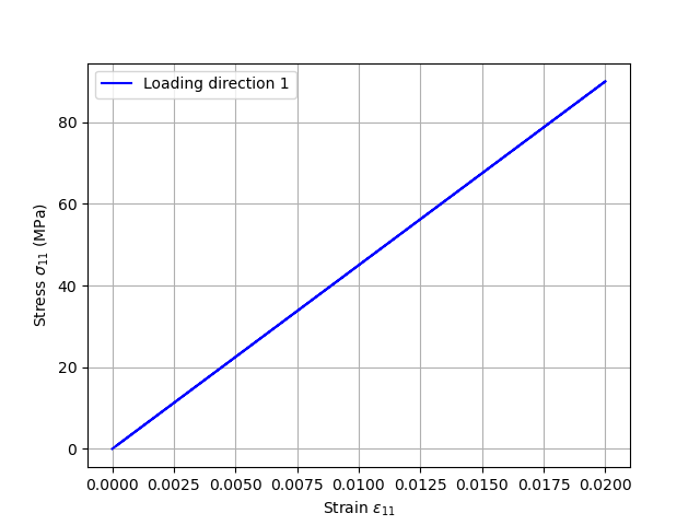
Plotting the results

We plot the stress-strain curve in the loading direction (direction 1).

outputfile_macro = os.path.join(path_results, "results_ELIST_global-0.txt")

fig = plt.figure()

e11, e22, e33, e12, e13, e23, s11, s22, s33, s12, s13, s23 = np.loadtxt(
    outputfile_macro,
    usecols=(8, 9, 10, 11, 12, 13, 14, 15, 16, 17, 18, 19),
    unpack=True,
)

plt.grid(True)
plt.xlabel(r"Strain $\varepsilon_{11}$")
plt.ylabel(r"Stress $\sigma_{11}$ (MPa)")
plt.plot(e11, s11, c="blue", label="Loading direction 1")
plt.legend(loc="best")

plt.show()