Note
Go to the end to download the full example code.
Hyperelastic models - use the API
In this example, we compare three hyperelastic constitutive laws. Each model is run for uniaxial tension (UT), equibiaxial tension (ET), and pure shear (PS).
We present one section per model.
# sphinx_gallery_thumbnail_number = 1

from math import fabs
import numpy as np
import pandas as pd
import simcoon as sim
import matplotlib.pyplot as plt
import os
from typing import NamedTuple, List, Tuple
from dataclasses import dataclass
from scipy.optimize import fsolve

# ###################################################################################
# Several hyperelastic isotropic materials are tested.
# They are compared to the well-know Traloar experimental data The following
# model are tested
#
# - The Neo-Hookean model
# - The Mooney-Rivlin model
# - The Isihara model
# - The Gent-Thomas model
#
# Considering the Neo-Hookean model, the strain energy function is expressed as:
#
# .. math::
#    W = \frac{\mu}{2}\left(\bar{I}_1 - 3\right) + \kappa\left( J\ln J - J + 1\right)
#
# The parameters are:
# 1. The shear coefficient :math:`\mu`,
# 2. The bulk compressibility :math:`\kappa`,
#
# Considering the Mooney-Rivlin model, the strain energy function is expressed as:
#
# .. math::
#    W = C_{10} \left(\bar{I}_1 -3\right) + C_{01} \left(\bar{I}_2 -3\right) + \kappa \left( J \ln J - J + 1 \right)
#
# The parameters are:
# 1. The first governing parameter :math:`c_{10}`,
# 2. The second governing parameter :math:`c_{01}`,
# 3. The bulk compressibility :math:`\kappa`,
#
# Considering the Isihara model, the strain energy function is expressed as:
#
# .. math::
#    W = C_{10} \left(\bar{I}_1 -3\right) + C_{20} \left(\bar{I}_1 -3\right)^2 + C_{01} \left(\bar{I}_2 -3\right) + \kappa \left( J \ln J - J +1 \right)
#
# The parameters are:
# 1. The first governing parameter :math:`c_{10}`,
# 2. The second governing parameter :math:`c_{20}`,
# 3. The third governing parameter :math:`c_{01}`,
# 4. The bulk compressibility :math:`\kappa`,
#
# Considering the Gent-Thomas model, the strain energy function is expressed as:
#
# .. math::
#    W = c_1 \left(\bar{I}_1 -3\right) + c_2 \ln \left( \frac{\bar{I}_2}{3}\right) + \kappa \left( J \ln J - J +1 \right)
#
# The parameters are:
# 1. The first governing parameter :math:`c_{1}`,
# 2. The second governing parameter :math:`c_{2}`,
# 3. The third governing parameter :math:`c_{01}`,
# 4. The bulk compressibility :math:`\kappa`,
#
# Considering the Swanson model, the strain energy function is expressed as:
#
# .. math::
#    W = \frac{3}{2} \sum_{i=1}^n \frac{A_i}{1+\alpha_i} \left(\frac{\bar{I}_1}{3}\right)^{1+\alpha_i} + \frac{3}{2} \sum_{i=1}^n \frac{B_i}{1+\beta_i} \left(\frac{\bar{I}_2}{3}\right)^{1+\beta_i} + \kappa \left( J \ln J - J +1 \right)
#
# The parameters are,
# 1. The size of the series :math:`n`,
# 2. The bulk compressibility :math:`\kappa`,
# Then for each serie :math:`i`:
# 1. The first shear modulus :math:`A_{i}`,
# 2. The second shear modulus :math:`B_{i}`,
# 3. The first exponent :math:`\alpha_{i}`,
# 4. The second exponent :math:`\beta_{i}`,
Data structures for material models and loading cases
In this section we define a small helper structures used throughout the example to organize material parameters and the data associated with each loading case.
loading_case is a NamedTuple describing one deformation or test scenario.
It contains the following fields:
name: a short label for the loading type (e.g. “uniaxial”).pathfile: the file path where the analytical or numerical results for this loading case are stored.comparison: a list of tuples, each holding two pandas Series (typically experimental vs analytical stress–stretch data) that can be plotted or analyzed together.
These lightweight structures help keep the code clean and make the processing and comparison loops later in the example more readable.
class loading_case(NamedTuple):
    name: str
    lambda_max: float
    pathfile: str
    comparison: List[Tuple[pd.Series, pd.Series]]
Reading experimental and analytical Treloar data
This example demonstrates how to load two datasets used for comparing experimental results with analytical predictions of the Treloar model.
The data files are stored in the comparison directory:
Treloar.txtcontains experimental measurements from Treloar’s classical rubber elasticity experiments. Each row lists the principal stretch ratios (lambda_1, lambda_2, lambda_3) together with the corresponding measured stresses (P1_MPa, P2_MPa, P3_MPa).
The files are space-separated, so pandas.read_csv is instructed
to use a whitespace separator (sep=r"\s+"). The column names are
supplied explicitly because the files contain header lines that we
ignore with header=0. Each dataset is read into its own pandas
DataFrame for further processing and comparison in later sections.
path_data = "comparison"
comparison_file_exp = "Treloar.txt"
comparison_exp = path_data + "/" + comparison_file_exp

df_exp = pd.read_csv(
    comparison_exp,
    sep=r"\s+",
    engine="python",
    names=["lambda_1", "P1_MPa", "lambda_2", "P2_MPa", "lambda_3", "P3_MPa"],
    header=0,
)
Defining the loading cases for comparison Here we create the different deformation modes used to compare the experimental Treloar data with the analytical predictions.
Each loading case is represented by a loading_case NamedTuple that
contains the following fields:
name: a short identifier for the deformation mode.pathfile: the file describing the deformation path (used later for analytical evaluations).comparison: a list of pairs of pandas Series, typically (experimental data, analytical data), for the stress component that corresponds to this loading mode.
The three classical Treloar tests included here are:
Uniaxial tension (UT): Uses the stretch \(\lambda_1\) and the corresponding stress component \(P_1\).
Pure shear (PS): Uses the stretch \(\lambda_2\) and the corresponding stress component \(P_2\).
Equi-biaxial tension (ET): Uses the stretch \(\lambda_3\) and the corresponding stress component \(P_3\).
These loading cases are gathered into the list loading_cases for
convenient iteration in subsequent plotting or evaluation steps.
Uniaxial_tension = loading_case(
    name="UT",
    lambda_max=7.65,
    pathfile="path_UT.txt",
    comparison=[
        (df_exp["lambda_1"], df_exp["P1_MPa"]),
    ],
)
Pure_shear = loading_case(
    name="PS",
    lambda_max=5.0,
    pathfile="path_PS.txt",
    comparison=[
        (df_exp["lambda_2"], df_exp["P2_MPa"]),
    ],
)
Equi_biaxial_tension = loading_case(
    name="ET",
    lambda_max=4.5,
    pathfile="path_ET.txt",
    comparison=[
        (df_exp["lambda_3"], df_exp["P3_MPa"]),
    ],
)

loading_cases = [Uniaxial_tension, Pure_shear, Equi_biaxial_tension]
- Material model parameters organized by loading case
Parameters are provided for each model and each loading case (UT, ET, PS)
This dictionary can be used to dynamically assign parameters to the models when looping over loading cases in the plotting and simulation sections.
Data are taken from Hyperelastic models for rubber-like materials: Consistent tangent operators and suitability for Treloar’s data Steinmann, P., Mokarram Hossain, Gunnar Possart September 2012 Archive of Applied Mechanics 82(9) DOI: 10.1007/s00419-012-0610-z
_bulk_neo = 1000.0
_bulk_mooney = 4000.0
_bulk_isihara = 4000.0
_bulk_gent = 4000.0

parameters_by_case = {
    "UT": {
        "NEOHC": [0.5673, _bulk_neo],
        "MOORI": [0.2588, -0.0449, _bulk_mooney],
        "ISHAH": [0.1161, 0.0136, 0.0114, _bulk_isihara],
        "GETHH": [0.2837, 2.81e-11, _bulk_gent],
    },
    "PS": {
        "NEOHC": [0.3360, _bulk_neo],
        "MOORI": [0.2348, -0.065, _bulk_mooney],
        "ISHAH": [0.1601, 0.0037, 0.0031, _bulk_isihara],
        "GETHH": [0.1629, 0.0376, _bulk_gent],
    },
    "ET": {
        "NEOHC": [0.4104, _bulk_neo],
        "MOORI": [0.1713, 0.0047, _bulk_mooney],
        "ISHAH": [0.1993, 0.0015, 0.0013, _bulk_isihara],
        "GETHH": [0.2052, 2.22e-14, _bulk_gent],
    },
}
Swanson model parameters has more complex coefficients (A, B, alpha, beta) for each loading case. These are kept in a separate dictionary.
Swanson_params = {
    "UT": {
        "A": [2.83e-3, 2.82e-13],
        "B": [1.871e-13, 0.4643],
        "alpha": [1.684, 9.141],
        "beta": [-0.4302, 0.7882],
    },
    "PS": {
        "A": [0.0676, 3.266e-11],
        "B": [0.2861, 0.0267],
        "alpha": [0.2687, 9.131],
        "beta": [-0.4683, 0.7157],
    },
    "ET": {
        "A": [0.21, 0.0074],
        "B": [0.1036, 0.266],
        "alpha": [-1833.0, 1.429],
        "beta": [-6.634, -0.623],
    },
}
We flatten and insert Swanson (“SWANS”) parameters into parameters_by_case
N_series = 2
bulk_swanson = 4000.0

for case_name in ("UT", "PS", "ET"):
    A = Swanson_params[case_name]["A"]
    B = Swanson_params[case_name]["B"]
    alpha = Swanson_params[case_name]["alpha"]
    beta = Swanson_params[case_name]["beta"]

    swanson_list = [N_series, bulk_swanson]
    for j in range(N_series):
        swanson_list += [A[j], B[j], alpha[j], beta[j]]

    # add to existing parameters_by_case for this loading case
    parameters_by_case[case_name]["SWANS"] = swanson_list
Here the derivatives of the strain energy function \(\frac{\partial W}{\partial \bar{I}_1}, \frac{\partial W}{\partial \bar{I}_2}, \frac{\partial W}{\partial J}\) are determined for each model.
def dW(model_name, parameters, b, J=0.0):
    if abs(J) < 1.0e-12:
        J = np.sqrt(np.linalg.det(b))

    I_bar = sim.isochoric_invariants(b, J)
    I1_bar = I_bar[0].item()
    I2_bar = I_bar[1].item()

    if model_name == "NEOHC":
        mu = parameters[0]
        kappa = parameters[1]
        dWdI_1_bar = 0.5 * mu
        dWdI_2_bar = 0.0
        dUdJ = kappa * np.log(J)

    elif model_name == "MOORI":
        C_10 = parameters[0]
        C_01 = parameters[1]
        kappa = parameters[2]
        dWdI_1_bar = C_10
        dWdI_2_bar = C_01
        dUdJ = kappa * np.log(J)

    elif model_name == "ISHAH":
        C_10 = parameters[0]
        C_20 = parameters[1]
        C_01 = parameters[2]
        kappa = parameters[3]
        dWdI_1_bar = C_10 + 2.0 * C_20 * (I1_bar - 3.0) * C_01 * (I2_bar - 3.0)
        dWdI_2_bar = C_20 * C_01 * pow((I1_bar - 3.0), 2.0)
        dUdJ = kappa * np.log(J)

    elif model_name == "SWANS":
        # Swanson model (series form)
        # parameters layout: [N_series, kappa, A1, B1, alpha1, beta1, A2, B2, alpha2, beta2, ...]
        N_series = int(parameters[0])
        kappa = parameters[1]

        # collect series coefficients
        A = [0.0] * N_series
        B = [0.0] * N_series
        alpha = [0.0] * N_series
        beta = [0.0] * N_series

        for i in range(N_series):
            base = 2 + i * 4
            A[i] = parameters[base]
            B[i] = parameters[base + 1]
            alpha[i] = parameters[base + 2]
            beta[i] = parameters[base + 3]

        dWdI_1_bar = 0.0
        dWdI_2_bar = 0.0

        # sum contributions from each series term
        for i in range(N_series):
            # use I_bar[0] = \bar{I}_1, I_bar[1] = \bar{I}_2
            dWdI_1_bar += 0.5 * A[i] * ((I1_bar / 3.0) ** (alpha[i]))
            dWdI_2_bar += 0.5 * B[i] * ((I2_bar / 3.0) ** (beta[i]))

        dUdJ = kappa * np.log(J)

    return (dWdI_1_bar, dWdI_2_bar, dUdJ)
Loading case functions to compute PK1
Here we add a decorator and the functions ut_, ps_ and et_ to compute PK1 for the
uniaxial tension, pure shear and equibiaxial tension cases
Note: Each function uses a root-finding algorithm to determine the transverse stretch that satisfies the equilibrium condition (zero transverse stress) for the given axial stretch. - For uniaxial tension, we apply stretch \(\lambda_1\) in the direction \(1\) and solve for \(\lambda_t\) in directions \(2\) and \(3\) such that \(\sigma_{22}\) = \(\sigma_{33}\) = 0. - For pure shear, we apply stretch \(\lambda_1\) in the direction \(1\) and solve for \(\lambda_t\) such that \(\sigma_{22}\) = 0, while keeping \(\lambda_3\) = 1. - For equibiaxial tension, we apply stretch \(\lambda_1\) in the directions \(1\) and \(2\) and solve for \(\lambda_t\) such that \(\sigma_{33}\) = 0.
CASE_DISPATCH = {}


def register_case(case_name: str):
    def decorator(func):
        CASE_DISPATCH[case_name] = func
        return func

    return decorator


def generic_case(lam1_array, case_name, model_name, parameters_by_case):
    """
    Generic solver for UT, PS, ET loading cases. Registered below for each case.
    """
    PK1 = []
    lam_t_guess = 1.0

    for lam1 in lam1_array:

        def equilibrium(lam_t):
            lt = lam_t[0]
            if case_name == "UT":
                F = np.diag([lam1, lt, lt])
                J = lam1 * lt**2
            elif case_name == "PS":
                F = np.diag([lam1, lt, 1.0])
                J = lam1 * lt
            elif case_name == "ET":
                F = np.diag([lam1, lam1, lt])
                J = lam1**2 * lt
            else:
                raise ValueError(f"Unknown case '{case_name}'")

            b = sim.L_Cauchy_Green(F)

            dWdI_1_bar, dWdI_2_bar, dUdJ = dW(
                model_name, parameters_by_case[case_name][model_name], b, J
            )

            sigma_iso = sim.sigma_iso_hyper_invariants(
                float(dWdI_1_bar), float(dWdI_2_bar), b, J, False
            )
            sigma_vol = sim.sigma_vol_hyper(dUdJ, b, J, False)
            sigma = sigma_iso + sigma_vol

            if case_name == "UT":
                return 0.5 * (sigma[1, 1] + sigma[2, 2])
            if case_name == "PS":
                return sigma[1, 1]
            # ET
            return sigma[2, 2]

        lam_t = fsolve(equilibrium, lam_t_guess)[0]
        lam_t_guess = lam_t

        # final state
        if case_name == "UT":
            F = np.diag([lam1, lam_t, lam_t])
            J = lam1 * lam_t**2
        elif case_name == "PS":
            F = np.diag([lam1, lam_t, 1.0])
            J = lam1 * lam_t
        else:  # ET
            F = np.diag([lam1, lam1, lam_t])
            J = lam1**2 * lam_t

        b = sim.L_Cauchy_Green(F)

        dWdI_1_bar, dWdI_2_bar, dUdJ = dW(
            model_name, parameters_by_case[case_name][model_name], b, J
        )

        sigma_iso = sim.sigma_iso_hyper_invariants(
            float(dWdI_1_bar), float(dWdI_2_bar), b, J, False
        )
        sigma_vol = sim.sigma_vol_hyper(dUdJ, b, J, False)
        sigma = sigma_iso + sigma_vol

        PK1.append(sigma[0, 0] / lam1)

    return np.array(PK1)


# register the same implementation for the three cases
for _case in ("UT", "PS", "ET"):
    register_case(_case)(generic_case)
This function uses the CASE_DISPATCH dictionary to call the appropriate function based on the case_name provided.
def run_case(
    lam1_array,
    case_name,
    model_name,
    parameters_by_case,
):
    try:
        func = CASE_DISPATCH[case_name]
    except KeyError:
        raise ValueError(f"No implementation registered for case '{case_name}'")

    return func(
        lam1_array,
        case_name,
        model_name,
        parameters_by_case,
    )
Plot each model separately For each hyperelastic model, we create one figure with three subplots: Uniaxial Tension (UT), Pure Shear (PS), and Equi-biaxial Tension (ET). The model parameters are automatically retrieved from parameters_by_case. Treloar experimental data and analytical results are plotted for comparison.
models_to_plot = ["NEOHC", "MOORI", "ISHAH", "GETHH", "SWANS"]
model_colors = {"NEOHC": "blue", "MOORI": "orange", "ISHAH": "green", "SWANS": "red"}
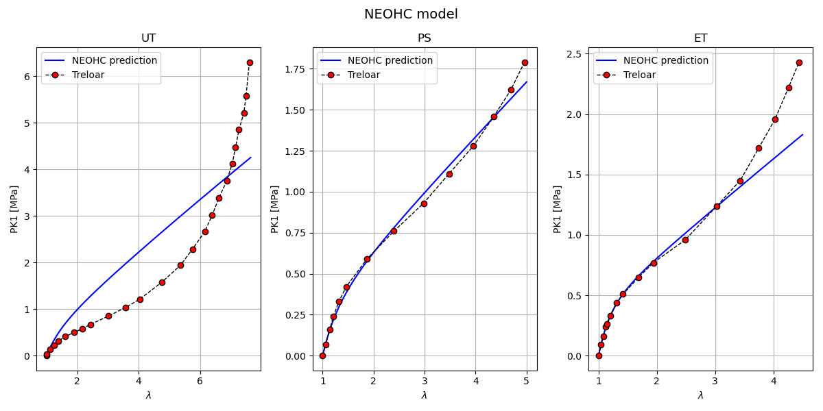
Neo-Hookean model plotting Here we plot the Neo-Hookean model predictions against the Treloar experimental data for each loading case.
Inputs: parameters_by_case[‘UT’|’PS’|’ET’][‘NEOHC’]: model parameters [mu, kappa] comparison/Treloar.txt: experimental Treloar data (lambda, P_MPa) Simcoon Python bindings (simcoon) for stress helpers
Outputs: A figure with 3 subplots (UT, PS, ET) showing PK1_11 vs lambda. Overlaid Treloar experimental points for visual comparison.
Notes: The script computes isochoric and volumetric stress contributions and assembles the total Cauchy stress used to compute PK1_11.
Expected figure: Left: Uniaxial tension PK1_11 vs lambda with Treloar markers Middle: Pure shear PK1_11 vs lambda with Treloar markers Right: Equibiaxial tension PK1_11 vs lambda with Treloar markers
fig, axes = plt.subplots(1, 3, figsize=(12, 6))

model_name = "NEOHC"
for i, case in enumerate(loading_cases):
    # Retrieve model parameters for this loading case
    params = parameters_by_case[case.name][model_name]

    lambda_1 = np.linspace(1.0, case.lambda_max, 500)
    PK1_11 = run_case(
        lambda_1,
        case.name,
        model_name,
        parameters_by_case,
    )

    # Plot model prediction
    axes[i].plot(
        lambda_1,
        PK1_11,
        color=model_colors[model_name],
        label=f"{model_name} prediction",
    )

    # Plot Treloar experimental data
    axes[i].plot(
        case.comparison[0][0],
        case.comparison[0][1],
        linestyle="--",
        marker="o",
        color="black",
        lw=1,
        markerfacecolor="red",
        markeredgecolor="black",
        label="Treloar",
    )

    # Formatting
    axes[i].set_xlabel(r"$\lambda$")
    axes[i].set_ylabel("PK1 [MPa]")
    axes[i].set_title(case.name)
    axes[i].grid(True)
    axes[i].legend()

fig.suptitle(f"{model_name} model", fontsize=14)
fig.tight_layout()
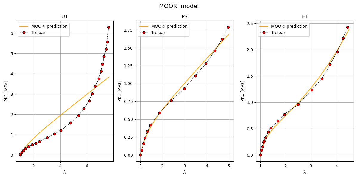
Mooney-Rivlin model plotting Here we plot the Mooney-Rivlin model predictions against the Treloar experimental data for each loading case.
Sphinx-Gallery notes Inputs: parameters_by_case[‘UT’|’PS’|’ET’][‘MOORI’]: model parameters [C10, C01, kappa] comparison/Treloar.txt: experimental Treloar data (lambda, P_MPa) Simcoon Python bindings (simcoon) for stress helpers
Outputs: A figure with 3 subplots (UT, PS, ET) showing PK1_11 vs lambda. Overlaid Treloar experimental points for visual comparison.
Notes: The Mooney-Rivlin model uses two isochoric invariants; the script passes the computed derivatives to the simcoon stress helper.
fig, axes = plt.subplots(1, 3, figsize=(12, 6))

model_name = "MOORI"
for i, case in enumerate(loading_cases):
    # Retrieve model parameters for this loading case
    params = parameters_by_case[case.name][model_name]

    lambda_1 = np.linspace(1.0, case.lambda_max, 500)
    PK1_11 = run_case(
        lambda_1,
        case.name,
        model_name,
        parameters_by_case,
    )

    # Plot model prediction
    axes[i].plot(
        lambda_1,
        PK1_11,
        color=model_colors[model_name],
        label=f"{model_name} prediction",
    )

    # Plot Treloar experimental data
    axes[i].plot(
        case.comparison[0][0],
        case.comparison[0][1],
        linestyle="--",
        marker="o",
        color="black",
        lw=1,
        markerfacecolor="red",
        markeredgecolor="black",
        label="Treloar",
    )

    # Formatting
    axes[i].set_xlabel(r"$\lambda$")
    axes[i].set_ylabel("PK1 [MPa]")
    axes[i].set_title(case.name)
    axes[i].grid(True)
    axes[i].legend()

fig.suptitle(f"{model_name} model", fontsize=14)
fig.tight_layout()
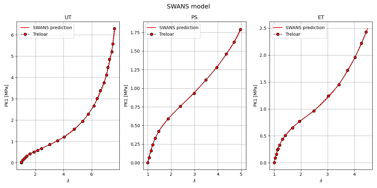
Swanson model plotting (N, K, then for each series: A, B, alpha, beta) Sphinx-Gallery notes Inputs: parameters_by_case[case][‘SWANS’]: flattened series parameters [N_series, kappa, A1, B1, alpha1, beta1, …] comparison/Treloar.txt: experimental Treloar data (lambda, P_MPa) Simcoon Python bindings (simcoon) for stress helpers
Outputs: A figure with 3 subplots (UT, PS, ET) showing PK1_11 vs lambda. Overlaid Treloar experimental points for visual comparison.
Notes: The Swanson model sums series contributions for the isochoric terms; ensure N_series matches the number of series coefficients provided.
fig, axes = plt.subplots(1, 3, figsize=(12, 6))

model_name = "SWANS"
N_series = 2
bulk_swanson = 4000.0  # bulk modulus

for i, case in enumerate(loading_cases):
    # Flatten parameters in solver order: N, K, then series 1..N: A, B, alpha, beta
    swanson_list = [N_series, bulk_swanson]
    for j in range(N_series):
        swanson_list += [
            Swanson_params[case.name]["A"][j],
            Swanson_params[case.name]["B"][j],
            Swanson_params[case.name]["alpha"][j],
            Swanson_params[case.name]["beta"][j],
        ]

    lambda_1 = np.linspace(1.0, case.lambda_max, 500)
    PK1_11 = run_case(
        lambda_1,
        case.name,
        model_name,
        parameters_by_case,
    )

    # Plot model prediction
    axes[i].plot(
        lambda_1,
        PK1_11,
        color=model_colors[model_name],
        label=f"{model_name} prediction",
    )

    # Plot Treloar experimental data
    axes[i].plot(
        case.comparison[0][0],
        case.comparison[0][1],
        linestyle="--",
        marker="o",
        color="black",
        lw=1,
        markerfacecolor="red",
        markeredgecolor="black",
        label="Treloar",
    )

    # Formatting
    axes[i].set_xlabel(r"$\lambda$")
    axes[i].set_ylabel("PK1 [MPa]")
    axes[i].set_title(case.name)
    axes[i].grid(True)
    axes[i].legend()

fig.suptitle(f"{model_name} model", fontsize=14)
fig.tight_layout()

plt.legend()
plt.show()
Total running time of the script: (0 minutes 1.249 seconds)