2 phase composite homogenization example

This tutorial studies the evolution of the mechanical properties of a composite material considering spherical and ellipsoidal reinforcements.

import numpy as np
from simcoon import simmit as sim
import matplotlib.pyplot as plt
import os

In this tutorial we will study mechanical properties of a 2-phase composite material considering spherical reinforcement. We will also explore the effect of inclusion aspect ratio on both the Eshelby tensor and the effective properties.

First we define the number of state variables (if any) at the macroscopic level and the material properties.

nstatev = 0  # None here

nphases = 2  # Number of phases
num_file = 0  # Index of the file that contains the subphases
int1 = 50  # Number of integration points along the long axis
int2 = 50  # Number of integration points along the lat axis
n_matrix = 0  # Phase number for the matrix

props = np.array([nphases, num_file, int1, int2, n_matrix], dtype="float")

There is a possibility to consider a misorientation between the test frame of reference and the composite material orientation, using Euler angles with the z–x–z convention. The stiffness tensor will be returned in the test frame of reference.

We also specify which micromechanical scheme will be used:

• MIMTN → Mori-Tanaka scheme

• MISCN → Self-consistent scheme

psi_rve = 0.0
theta_rve = 0.0
phi_rve = 0.0

umat_name = "MIMTN"  # Micromechanical scheme (Mori-Tanaka here)

Run the simulation to obtain the effective isotropic elastic properties. Since both phases are isotropic and the reinforcements are spherical, the result is also isotropic.

L_eff = sim.L_eff(umat_name, props, nstatev, psi_rve, theta_rve, phi_rve)
p = sim.L_iso_props(L_eff).flatten()
np.set_printoptions(precision=3, suppress=True)

print("L_eff = ", L_eff)
print("Effective isotropic properties (E, nu):", p)

L_eff =  [[3622.978  859.796  859.796    0.       0.      -0.   ]
 [ 859.796 3622.978  859.796   -0.       0.       0.   ]
 [ 859.796  859.796 3622.978    0.       0.      -0.   ]
 [   0.      -0.       0.    1381.591    0.       0.   ]
 [   0.       0.       0.       0.    1381.591    0.   ]
 [  -0.       0.      -0.       0.       0.    1381.591]]
Effective isotropic properties (E, nu): [3293.16     0.192]

Note: Even though both materials share the same Poisson ratio, the stiffness mismatch leads to a different effective Poisson ratio.

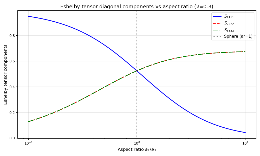
Effect of aspect ratio on Eshelby tensor components

The Eshelby tensor \(\mathbf{S}\) relates the constrained strain inside an ellipsoidal inclusion to the eigenstrain. It depends on the inclusion shape and the matrix Poisson ratio. Let’s visualize how its components vary with aspect ratio.

nu = 0.3  # Poisson ratio of the matrix

aspect_ratios = np.logspace(-1, 1, 50)  # From 0.1 to 10
S_11 = []
S_22 = []
S_33 = []

for ar in aspect_ratios:
    if ar > 1:
        S = sim.Eshelby_prolate(nu, ar)
    else:
        S = sim.Eshelby_oblate(nu, ar)
    S_11.append(S[0, 0])
    S_22.append(S[1, 1])
    S_33.append(S[2, 2])

fig, ax = plt.subplots(figsize=(10, 6))
ax.semilogx(aspect_ratios, S_11, "b-", label=r"$S_{1111}$", linewidth=2)
ax.semilogx(aspect_ratios, S_22, "r--", label=r"$S_{2222}$", linewidth=2)
ax.semilogx(aspect_ratios, S_33, "g-.", label=r"$S_{3333}$", linewidth=2)
ax.axvline(x=1, color="k", linestyle=":", alpha=0.5, label="Sphere (ar=1)")
ax.set_xlabel("Aspect ratio $a_1/a_3$", fontsize=12)
ax.set_ylabel("Eshelby tensor components", fontsize=12)
ax.set_title(
    f"Eshelby tensor diagonal components vs aspect ratio ($\\nu$={nu})", fontsize=14
)
ax.legend(fontsize=11)
ax.grid(True, alpha=0.3)
plt.tight_layout()
plt.show()