Note
Go to the end to download the full example code.
Parameter Identification for Mooney-Rivlin Hyperelastic Material
This example demonstrates inverse parameter identification for hyperelastic materials using experimental stress-strain data. We identify the Mooney-Rivlin model parameters from Treloar’s classical rubber elasticity experiments.
Optimization: scipy.optimize.differential_evolution (global optimizer) Cost function: Mean Squared Error on stress (sklearn.metrics.mean_squared_error) Forward model: simcoon hyperelastic stress functions
See also
examples/hyperelasticity/hyperelastic_umat_identification.py solves the
same problem with the deployable MOORI UMAT (via sim.solver) and
Simcoon’s identification API (sim.identification + sim.calc_cost).
This analytical version is fast and exposes the physics; that one exercises
the production UMAT and the library cost function.
import numpy as np
import pandas as pd
import matplotlib.pyplot as plt
from scipy.optimize import differential_evolution, fsolve
from sklearn.metrics import mean_squared_error
from simcoon import simmit as sim
import os
Methodology Overview
Inverse Problem Formulation
Parameter identification is an inverse problem: given experimental observations (stress-strain data), we seek the material parameters that minimize the discrepancy between model predictions and experiments.
The optimization problem is:
where \(\boldsymbol{\theta}\) are the material parameters and \(\mathcal{L}\) is the cost function.
Cost Function: Stress-Based MSE
We use the Mean Squared Error (MSE) computed on the first Piola-Kirchhoff stress \(P_{11}\):
This stress-based metric directly measures the model’s ability to predict mechanical response, which is the primary quantity of interest in constitutive modeling.
Why Differential Evolution?
We use scipy.optimize.differential_evolution because:
Global optimization: Unlike gradient-based methods, it explores the entire parameter space and avoids local minima
Derivative-free: No gradients required, robust for non-smooth objectives
Bounded search: Natural handling of physical parameter constraints
Robustness: Less sensitive to initial guess compared to local methods
For hyperelastic models, the cost function landscape can be non-convex, making global optimization essential for reliable parameter identification.
Mooney-Rivlin Constitutive Model
The Mooney-Rivlin model is a phenomenological hyperelastic model widely used for rubber-like materials. The strain energy function is:
where:
\(\bar{I}_1, \bar{I}_2\) are the first and second isochoric invariants of the left Cauchy-Green tensor \(\mathbf{b} = \mathbf{F}\mathbf{F}^T\)
\(C_{10}, C_{01}\) are the material parameters to identify
\(U(J) = \kappa(J \ln J - J + 1)\) is the volumetric contribution
\(\kappa\) is the bulk modulus (fixed, assuming near-incompressibility)
The Cauchy stress is computed as:
where simcoon provides sigma_iso_hyper_invariants and sigma_vol_hyper
to compute these contributions from the strain energy derivatives:
Experimental Data: Treloar’s Rubber Experiments
L.R.G. Treloar (1944) performed classical experiments on vulcanized rubber under three loading conditions:
Uniaxial Tension (UT): \(\lambda_1 = \lambda, \lambda_2 = \lambda_3 = \lambda_t\)
Pure Shear (PS): \(\lambda_1 = \lambda, \lambda_2 = \lambda_t, \lambda_3 = 1\)
Equibiaxial Tension (ET): \(\lambda_1 = \lambda_2 = \lambda, \lambda_3 = \lambda_t\)
where \(\lambda_t\) is the transverse stretch determined by equilibrium (zero transverse stress). The data provides stretch \(\lambda\) and the corresponding first Piola-Kirchhoff stress \(P_{11}\) [MPa].
def load_treloar_data(filepath: str) -> pd.DataFrame:
    """
    Load Treloar experimental data.

    The file contains columns for three loading cases:
    - lambda_1, P1_MPa: Uniaxial tension
    - lambda_2, P2_MPa: Pure shear
    - lambda_3, P3_MPa: Equibiaxial tension

    Parameters
    ----------
    filepath : str
        Path to Treloar.txt data file

    Returns
    -------
    pd.DataFrame
        Experimental data with columns for each loading case
    """
    df = pd.read_csv(
        filepath,
        sep=r"\s+",
        engine="python",
        names=["lambda_1", "P1_MPa", "lambda_2", "P2_MPa", "lambda_3", "P3_MPa"],
        header=0,
    )
    return df
Forward Model: Stress Prediction using simcoon
The forward model computes the first Piola-Kirchhoff stress for given material parameters and stretch values. This is the core function that will be called repeatedly during optimization.
Key steps:
For each stretch \(\lambda_1\), solve for the transverse stretch \(\lambda_t\) that satisfies equilibrium (zero transverse stress)
Construct the deformation gradient \(\mathbf{F}\)
Compute the left Cauchy-Green tensor \(\mathbf{b} = \mathbf{F}\mathbf{F}^T\) using
sim.L_Cauchy_Green(F)Compute strain energy derivatives for Mooney-Rivlin
Compute Cauchy stress using
sim.sigma_iso_hyper_invariantsandsim.sigma_vol_hyperConvert to first Piola-Kirchhoff stress: \(P_{11} = \sigma_{11}/\lambda_1\)
def mooney_rivlin_pk1_stress(
    C10: float,
    C01: float,
    kappa: float,
    lambda_array: np.ndarray,
    loading_case: str = "UT",
) -> np.ndarray:
    """
    Compute first Piola-Kirchhoff stress for Mooney-Rivlin material.

    Uses simcoon's hyperelastic stress functions to compute the Cauchy stress
    from the strain energy derivatives, then converts to PK1 stress.

    Parameters
    ----------
    C10 : float
        First Mooney-Rivlin parameter [MPa]
    C01 : float
        Second Mooney-Rivlin parameter [MPa]
    kappa : float
        Bulk modulus for volumetric response [MPa]
    lambda_array : np.ndarray
        Array of principal stretch values in the loading direction
    loading_case : str
        Type of loading: "UT" (uniaxial tension), "PS" (pure shear),
        or "ET" (equibiaxial tension)

    Returns
    -------
    np.ndarray
        First Piola-Kirchhoff stress P_11 [MPa]
    """
    PK1_stress = []
    lambda_t_guess = 1.0  # Initial guess for transverse stretch

    for lam in lambda_array:
        # -----------------------------------------------------------------
        # Step 1: Find transverse stretch satisfying equilibrium
        # -----------------------------------------------------------------
        def equilibrium_residual(lambda_t_vec):
            """Residual function for finding equilibrium transverse stretch."""
            lt = lambda_t_vec[0]

            # Construct deformation gradient based on loading case
            if loading_case == "UT":
                # Uniaxial: F = diag(lambda, lambda_t, lambda_t)
                F = np.diag([lam, lt, lt])
                J = lam * lt**2
            elif loading_case == "PS":
                # Pure shear: F = diag(lambda, lambda_t, 1)
                F = np.diag([lam, lt, 1.0])
                J = lam * lt
            elif loading_case == "ET":
                # Equibiaxial: F = diag(lambda, lambda, lambda_t)
                F = np.diag([lam, lam, lt])
                J = lam**2 * lt
            else:
                raise ValueError(f"Unknown loading case: {loading_case}")

            # Compute left Cauchy-Green tensor using simcoon
            b = sim.L_Cauchy_Green(F)

            # Mooney-Rivlin strain energy derivatives
            dW_dI1_bar = C10
            dW_dI2_bar = C01
            dU_dJ = kappa * np.log(J)

            # Compute Cauchy stress using simcoon functions
            sigma_iso = sim.sigma_iso_hyper_invariants(
                float(dW_dI1_bar), float(dW_dI2_bar), b, J, False
            )
            sigma_vol = sim.sigma_vol_hyper(dU_dJ, b, J, False)
            sigma = sigma_iso + sigma_vol

            # Return stress component that should be zero at equilibrium
            if loading_case == "UT":
                # sigma_22 = sigma_33 = 0
                return 0.5 * (sigma[1, 1] + sigma[2, 2])
            elif loading_case == "PS":
                # sigma_22 = 0
                return sigma[1, 1]
            else:  # ET
                # sigma_33 = 0
                return sigma[2, 2]

        # Solve for equilibrium transverse stretch
        lambda_t = fsolve(equilibrium_residual, lambda_t_guess, full_output=False)[0]
        lambda_t_guess = lambda_t  # Use as starting point for next iteration

        # -----------------------------------------------------------------
        # Step 2: Compute final stress state at equilibrium
        # -----------------------------------------------------------------
        if loading_case == "UT":
            F = np.diag([lam, lambda_t, lambda_t])
            J = lam * lambda_t**2
        elif loading_case == "PS":
            F = np.diag([lam, lambda_t, 1.0])
            J = lam * lambda_t
        else:  # ET
            F = np.diag([lam, lam, lambda_t])
            J = lam**2 * lambda_t

        b = sim.L_Cauchy_Green(F)

        # Strain energy derivatives
        dW_dI1_bar = C10
        dW_dI2_bar = C01
        dU_dJ = kappa * np.log(J)

        # Compute Cauchy stress
        sigma_iso = sim.sigma_iso_hyper_invariants(
            float(dW_dI1_bar), float(dW_dI2_bar), b, J, False
        )
        sigma_vol = sim.sigma_vol_hyper(dU_dJ, b, J, False)
        sigma = sigma_iso + sigma_vol

        # Convert Cauchy stress to PK1: P = J * sigma * F^{-T}
        # For diagonal F: P_11 = sigma_11 / lambda_1
        PK1_stress.append(sigma[0, 0] / lam)

    return np.array(PK1_stress)
Cost Function: Stress-Based Mean Squared Error
The cost function quantifies the discrepancy between model predictions and experimental data. We use MSE computed on the PK1 stress values.
Normalized MSE (NMSE):
When combining multiple loading cases with different stress magnitudes, we can normalize by the variance to ensure balanced weighting:
This ensures that loading cases with smaller stress magnitudes are not dominated by cases with larger stresses during combined fitting.
def cost_function_mse(
    params: np.ndarray,
    lambda_exp: np.ndarray,
    P_exp: np.ndarray,
    kappa: float,
    loading_case: str,
    normalize: bool = False,
) -> float:
    """
    Compute MSE cost between model prediction and experimental stress data.

    Parameters
    ----------
    params : np.ndarray
        Material parameters [C10, C01]
    lambda_exp : np.ndarray
        Experimental stretch values
    P_exp : np.ndarray
        Experimental PK1 stress values [MPa]
    kappa : float
        Fixed bulk modulus [MPa]
    loading_case : str
        Loading type ("UT", "PS", or "ET")
    normalize : bool
        If True, divide MSE by variance of experimental data

    Returns
    -------
    float
        MSE or NMSE value
    """
    C10, C01 = params

    try:
        # Predict stress using forward model
        P_model = mooney_rivlin_pk1_stress(C10, C01, kappa, lambda_exp, loading_case)

        # Compute MSE using sklearn
        mse = mean_squared_error(P_exp, P_model)

        if normalize:
            variance = np.var(P_exp)
            return mse / variance if variance > 1e-12 else mse
        return mse

    except Exception:
        # Return large cost if computation fails (e.g., numerical issues)
        return 1e10


def cost_function_combined(
    params: np.ndarray, data_dict: dict, kappa: float, normalize: bool = True
) -> float:
    """
    Combined cost function for simultaneous fitting to multiple loading cases.

    Parameters
    ----------
    params : np.ndarray
        Material parameters [C10, C01]
    data_dict : dict
        Dictionary mapping loading case names to (lambda, P) tuples
    kappa : float
        Fixed bulk modulus [MPa]
    normalize : bool
        If True, use NMSE for balanced weighting across cases

    Returns
    -------
    float
        Sum of (N)MSE values over all loading cases
    """
    total_cost = 0.0
    for case_name, (lambda_exp, P_exp) in data_dict.items():
        cost = cost_function_mse(params, lambda_exp, P_exp, kappa, case_name, normalize)
        total_cost += cost
    return total_cost
Parameter Identification using Differential Evolution
scipy.optimize.differential_evolution is a stochastic global optimizer
based on evolutionary algorithms. Key parameters:
bounds: Search space for each parameter
strategy: Mutation strategy (‘best1bin’ works well for most problems)
popsize: Population size (larger = more thorough search)
mutation: Mutation constant (controls exploration vs exploitation)
recombination: Crossover probability
polish: If True, refines result with L-BFGS-B (local optimizer)
def identify_parameters(
    lambda_exp: np.ndarray,
    P_exp: np.ndarray,
    kappa: float = 4000.0,
    loading_case: str = "UT",
    bounds: list = None,
    normalize: bool = False,
    seed: int = 42,
    verbose: bool = True,
) -> dict:
    """
    Identify Mooney-Rivlin parameters using differential evolution.

    Parameters
    ----------
    lambda_exp : np.ndarray
        Experimental stretch values
    P_exp : np.ndarray
        Experimental PK1 stress values [MPa]
    kappa : float
        Fixed bulk modulus [MPa] (default: 4000 for near-incompressibility)
    loading_case : str
        Loading type ("UT", "PS", or "ET")
    bounds : list
        Parameter bounds [(C10_min, C10_max), (C01_min, C01_max)]
    normalize : bool
        If True, use normalized MSE
    seed : int
        Random seed for reproducibility
    verbose : bool
        Print optimization progress

    Returns
    -------
    dict
        Optimized parameters and optimization results
    """
    if bounds is None:
        bounds = [(0.01, 2.0), (-1.0, 1.0)]

    if verbose:
        print(f"\n{'=' * 60}")
        print(f"Optimizing for {loading_case} loading case")
        print(f"{'=' * 60}")
        print(f"Parameter bounds: C10 in {bounds[0]}, C01 in {bounds[1]}")
        print(f"Bulk modulus (fixed): kappa = {kappa} MPa")

    result = differential_evolution(
        cost_function_mse,
        bounds=bounds,
        args=(lambda_exp, P_exp, kappa, loading_case, normalize),
        strategy="best1bin",
        maxiter=500,
        popsize=15,
        tol=1e-8,
        mutation=(0.5, 1.0),
        recombination=0.7,
        seed=seed,
        polish=True,  # Refine with L-BFGS-B
        disp=verbose,
    )

    C10_opt, C01_opt = result.x

    if verbose:
        print(f"\nOptimization completed!")
        print(f"  C10 = {C10_opt:.6f} MPa")
        print(f"  C01 = {C01_opt:.6f} MPa")
        print(f"  Final MSE = {result.fun:.6e} MPa^2")

    return {
        "C10": C10_opt,
        "C01": C01_opt,
        "kappa": kappa,
        "mse": result.fun,
        "success": result.success,
        "result": result,
    }


def identify_parameters_combined(
    data_dict: dict,
    kappa: float = 4000.0,
    bounds: list = None,
    normalize: bool = True,
    seed: int = 42,
    verbose: bool = True,
) -> dict:
    """
    Identify parameters by fitting to multiple loading cases simultaneously.

    Using NMSE (normalized MSE) ensures balanced contribution from each
    loading case, preventing cases with larger stress magnitudes from
    dominating the optimization.

    Parameters
    ----------
    data_dict : dict
        Dictionary {case_name: (lambda_exp, P_exp)} for each loading case
    kappa : float
        Fixed bulk modulus [MPa]
    bounds : list
        Parameter bounds [(C10_min, C10_max), (C01_min, C01_max)]
    normalize : bool
        If True, use NMSE (recommended for combined fitting)
    seed : int
        Random seed
    verbose : bool
        Print progress

    Returns
    -------
    dict
        Optimized parameters and results
    """
    if bounds is None:
        bounds = [(0.01, 2.0), (-1.0, 1.0)]

    if verbose:
        print(f"\n{'=' * 60}")
        print(f"Combined optimization for: {list(data_dict.keys())}")
        print(f"{'=' * 60}")
        print(f"Parameter bounds: C10 in {bounds[0]}, C01 in {bounds[1]}")
        print(f"Bulk modulus (fixed): kappa = {kappa} MPa")
        print(f"Using {'NMSE' if normalize else 'MSE'} for cost function")

    result = differential_evolution(
        cost_function_combined,
        bounds=bounds,
        args=(data_dict, kappa, normalize),
        strategy="best1bin",
        maxiter=500,
        popsize=15,
        tol=1e-8,
        mutation=(0.5, 1.0),
        recombination=0.7,
        seed=seed,
        polish=True,
        disp=verbose,
    )

    C10_opt, C01_opt = result.x

    if verbose:
        print(f"\nOptimization completed!")
        print(f"  C10 = {C10_opt:.6f} MPa")
        print(f"  C01 = {C01_opt:.6f} MPa")
        print(f"  Final combined cost = {result.fun:.6e}")

    return {
        "C10": C10_opt,
        "C01": C01_opt,
        "kappa": kappa,
        "cost": result.fun,
        "success": result.success,
        "result": result,
    }
Visualization Functions
def plot_fit_comparison(
    lambda_exp: np.ndarray,
    P_exp: np.ndarray,
    params: dict,
    loading_case: str,
    title: str = None,
    ax=None,
):
    """
    Plot experimental data vs model prediction.

    Parameters
    ----------
    lambda_exp : np.ndarray
        Experimental stretch values
    P_exp : np.ndarray
        Experimental PK1 stress values [MPa]
    params : dict
        Dictionary with 'C10', 'C01', 'kappa' keys
    loading_case : str
        Loading type
    title : str
        Plot title (optional)
    ax : matplotlib.axes.Axes
        Axes to plot on (creates new figure if None)

    Returns
    -------
    matplotlib.axes.Axes
        The axes with the plot
    """
    if ax is None:
        fig, ax = plt.subplots(figsize=(8, 6))

    # Model prediction on fine grid
    lambda_model = np.linspace(1.0, lambda_exp.max() * 1.02, 200)
    P_model = mooney_rivlin_pk1_stress(
        params["C10"], params["C01"], params["kappa"], lambda_model, loading_case
    )

    # Experimental data
    ax.plot(
        lambda_exp,
        P_exp,
        "o",
        markersize=8,
        markerfacecolor="red",
        markeredgecolor="black",
        label="Treloar experimental",
    )

    # Model prediction
    ax.plot(
        lambda_model,
        P_model,
        "-",
        linewidth=2,
        color="blue",
        label=f"Mooney-Rivlin (C10={params['C10']:.4f}, C01={params['C01']:.4f})",
    )

    ax.set_xlabel(r"Stretch $\lambda$ [-]", fontsize=12)
    ax.set_ylabel(r"PK1 Stress $P_{11}$ [MPa]", fontsize=12)
    ax.set_title(title or f"{loading_case} - Parameter Identification", fontsize=14)
    ax.legend(loc="upper left", fontsize=10)
    ax.grid(True, alpha=0.3)

    return ax
Main Execution
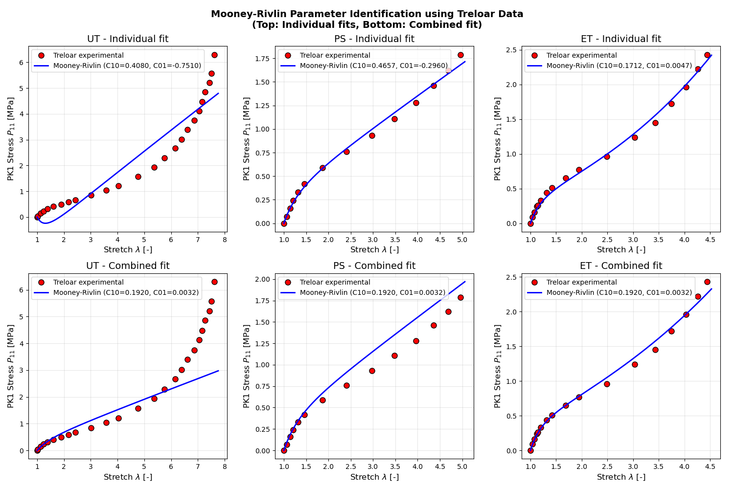
We demonstrate two identification strategies:
Individual fitting: Optimize parameters separately for each loading case
Combined fitting: Find a single parameter set that best fits all cases
The individual fits provide loading-case-specific parameters (useful for understanding material behavior), while combined fitting gives a universal parameter set for general use.
if __name__ == "__main__":
    # Locate data file relative to script
    # Try multiple approaches to find the data file (supports both direct
    # execution and Sphinx-Gallery which does not define __file__)
    data_filename = os.path.join("hyperelasticity", "comparison", "Treloar.txt")
    possible_paths = []

    # Try using __file__ if available
    try:
        script_dir = os.path.dirname(os.path.abspath(__file__))
        possible_paths.append(os.path.join(script_dir, "..", data_filename))
    except NameError:
        pass

    # Try relative to current working directory (Sphinx-Gallery context)
    possible_paths.append(os.path.join(os.getcwd(), "..", data_filename))
    possible_paths.append(os.path.join(os.getcwd(), "examples", data_filename))

    # Find first existing path
    data_path = None
    for path in possible_paths:
        if os.path.exists(path):
            data_path = path
            break

    if data_path is None:
        raise FileNotFoundError(
            f"Could not find Treloar.txt data file. Searched: {possible_paths}"
        )

    print("=" * 70)
    print(" MOONEY-RIVLIN PARAMETER IDENTIFICATION")
    print(" Using scipy.differential_evolution and sklearn.mean_squared_error")
    print("=" * 70)

    # -------------------------------------------------------------------------
    # Load and prepare experimental data
    # -------------------------------------------------------------------------
    df = load_treloar_data(data_path)
    print(f"\nLoaded Treloar data: {len(df)} data points")

    # Extract data for each loading case (remove NaN values)
    ut_mask = ~df["lambda_1"].isna() & ~df["P1_MPa"].isna()
    ps_mask = ~df["lambda_2"].isna() & ~df["P2_MPa"].isna()
    et_mask = ~df["lambda_3"].isna() & ~df["P3_MPa"].isna()

    lambda_ut = df.loc[ut_mask, "lambda_1"].values
    P_ut = df.loc[ut_mask, "P1_MPa"].values

    lambda_ps = df.loc[ps_mask, "lambda_2"].values
    P_ps = df.loc[ps_mask, "P2_MPa"].values

    lambda_et = df.loc[et_mask, "lambda_3"].values
    P_et = df.loc[et_mask, "P3_MPa"].values

    print(f"\nData summary:")
    print(
        f"  Uniaxial Tension (UT): {len(lambda_ut)} points, "
        f"lambda in [{lambda_ut.min():.2f}, {lambda_ut.max():.2f}]"
    )
    print(
        f"  Pure Shear (PS):       {len(lambda_ps)} points, "
        f"lambda in [{lambda_ps.min():.2f}, {lambda_ps.max():.2f}]"
    )
    print(
        f"  Equibiaxial (ET):      {len(lambda_et)} points, "
        f"lambda in [{lambda_et.min():.2f}, {lambda_et.max():.2f}]"
    )

    # Fixed bulk modulus (near-incompressible rubber)
    kappa = 4000.0

    # -------------------------------------------------------------------------
    # Individual fitting for each loading case
    # -------------------------------------------------------------------------
    print("\n" + "=" * 70)
    print(" INDIVIDUAL FITTING (one parameter set per loading case)")
    print("=" * 70)

    params_ut = identify_parameters(lambda_ut, P_ut, kappa, "UT", verbose=True)
    params_ps = identify_parameters(lambda_ps, P_ps, kappa, "PS", verbose=True)
    params_et = identify_parameters(lambda_et, P_et, kappa, "ET", verbose=True)

    # Reference values from literature (Steinmann et al., 2012)
    print("\n" + "-" * 70)
    print("Comparison with literature (Steinmann et al., 2012):")
    print("-" * 70)
    print(
        f"{'Case':<8} {'C10 (lit.)':<12} {'C10 (ident.)':<14} {'C01 (lit.)':<12} {'C01 (ident.)':<14}"
    )
    print("-" * 70)
    print(
        f"{'UT':<8} {0.2588:<12.4f} {params_ut['C10']:<14.4f} {-0.0449:<12.4f} {params_ut['C01']:<14.4f}"
    )
    print(
        f"{'PS':<8} {0.2348:<12.4f} {params_ps['C10']:<14.4f} {-0.065:<12.4f} {params_ps['C01']:<14.4f}"
    )
    print(
        f"{'ET':<8} {0.1713:<12.4f} {params_et['C10']:<14.4f} {0.0047:<12.4f} {params_et['C01']:<14.4f}"
    )

    # -------------------------------------------------------------------------
    # Combined fitting
    # -------------------------------------------------------------------------
    print("\n" + "=" * 70)
    print(" COMBINED FITTING (single parameter set for all loading cases)")
    print("=" * 70)

    data_combined = {
        "UT": (lambda_ut, P_ut),
        "PS": (lambda_ps, P_ps),
        "ET": (lambda_et, P_et),
    }

    params_combined = identify_parameters_combined(
        data_combined, kappa=kappa, normalize=True, verbose=True
    )

    # -------------------------------------------------------------------------
    # Visualization
    # -------------------------------------------------------------------------
    print("\n" + "=" * 70)
    print(" GENERATING PLOTS")
    print("=" * 70)

    fig, axes = plt.subplots(2, 3, figsize=(15, 10))

    # Row 1: Individual fits
    plot_fit_comparison(
        lambda_ut, P_ut, params_ut, "UT", title="UT - Individual fit", ax=axes[0, 0]
    )
    plot_fit_comparison(
        lambda_ps, P_ps, params_ps, "PS", title="PS - Individual fit", ax=axes[0, 1]
    )
    plot_fit_comparison(
        lambda_et, P_et, params_et, "ET", title="ET - Individual fit", ax=axes[0, 2]
    )

    # Row 2: Combined fit applied to all cases
    plot_fit_comparison(
        lambda_ut, P_ut, params_combined, "UT", title="UT - Combined fit", ax=axes[1, 0]
    )
    plot_fit_comparison(
        lambda_ps, P_ps, params_combined, "PS", title="PS - Combined fit", ax=axes[1, 1]
    )
    plot_fit_comparison(
        lambda_et, P_et, params_combined, "ET", title="ET - Combined fit", ax=axes[1, 2]
    )

    fig.suptitle(
        "Mooney-Rivlin Parameter Identification using Treloar Data\n"
        "(Top: Individual fits, Bottom: Combined fit)",
        fontsize=14,
        fontweight="bold",
    )
    plt.tight_layout()

    # -------------------------------------------------------------------------
    # Summary
    # -------------------------------------------------------------------------
    print("\n" + "=" * 70)
    print(" SUMMARY OF IDENTIFIED PARAMETERS")
    print("=" * 70)
    print(f"{'Case':<12} {'C10 [MPa]':>12} {'C01 [MPa]':>12} {'MSE [MPa^2]':>14}")
    print("-" * 52)
    print(
        f"{'UT':<12} {params_ut['C10']:>12.4f} {params_ut['C01']:>12.4f} {params_ut['mse']:>14.2e}"
    )
    print(
        f"{'PS':<12} {params_ps['C10']:>12.4f} {params_ps['C01']:>12.4f} {params_ps['mse']:>14.2e}"
    )
    print(
        f"{'ET':<12} {params_et['C10']:>12.4f} {params_et['C01']:>12.4f} {params_et['mse']:>14.2e}"
    )
    print("-" * 52)
    print(
        f"{'Combined':<12} {params_combined['C10']:>12.4f} {params_combined['C01']:>12.4f} {params_combined['cost']:>14.2e}"
    )
    print("=" * 70)

    print("\nNote: The combined fit uses NMSE (normalized MSE) which explains")
    print("the different cost magnitude compared to individual MSE values.")

    plt.show()
======================================================================
 MOONEY-RIVLIN PARAMETER IDENTIFICATION
 Using scipy.differential_evolution and sklearn.mean_squared_error
======================================================================

Loaded Treloar data: 25 data points

Data summary:
  Uniaxial Tension (UT): 25 points, lambda in [1.00, 7.61]
  Pure Shear (PS):       14 points, lambda in [1.00, 4.96]
  Equibiaxial (ET):      17 points, lambda in [1.00, 4.44]

======================================================================
 INDIVIDUAL FITTING (one parameter set per loading case)
======================================================================

============================================================
Optimizing for UT loading case
============================================================
Parameter bounds: C10 in (0.01, 2.0), C01 in (-1.0, 1.0)
Bulk modulus (fixed): kappa = 4000.0 MPa
differential_evolution step 1: f(x)= 0.4096615268469581
differential_evolution step 2: f(x)= 0.4096615268469581
differential_evolution step 3: f(x)= 0.3978263758640262
differential_evolution step 4: f(x)= 0.3978263758640262
differential_evolution step 5: f(x)= 0.39194853823940684
differential_evolution step 6: f(x)= 0.39194853823940684
differential_evolution step 7: f(x)= 0.390742001678335
differential_evolution step 8: f(x)= 0.390742001678335
differential_evolution step 9: f(x)= 0.38955535356791926
differential_evolution step 10: f(x)= 0.38955535356791926
differential_evolution step 11: f(x)= 0.38955535356791926
differential_evolution step 12: f(x)= 0.3895493503783034
differential_evolution step 13: f(x)= 0.3895134000272561
differential_evolution step 14: f(x)= 0.3895134000272561
differential_evolution step 15: f(x)= 0.3895134000272561
differential_evolution step 16: f(x)= 0.38951161523788896
differential_evolution step 17: f(x)= 0.38951044296197623
differential_evolution step 18: f(x)= 0.3895083336274455
differential_evolution step 19: f(x)= 0.38950807193905634
differential_evolution step 20: f(x)= 0.3895079700689561
differential_evolution step 21: f(x)= 0.3895079700689561
differential_evolution step 22: f(x)= 0.3895078172607434
differential_evolution step 23: f(x)= 0.3895078172607434
differential_evolution step 24: f(x)= 0.3895078172607434
differential_evolution step 25: f(x)= 0.3895078094426372
differential_evolution step 26: f(x)= 0.3895078094426372
differential_evolution step 27: f(x)= 0.3895078012254065
differential_evolution step 28: f(x)= 0.38950780048910943
differential_evolution step 29: f(x)= 0.38950780048910943
differential_evolution step 30: f(x)= 0.38950780044294975
differential_evolution step 31: f(x)= 0.38950780038681637
differential_evolution step 32: f(x)= 0.38950780038681637
Polishing solution with 'L-BFGS-B'

Optimization completed!
  C10 = 0.407989 MPa
  C01 = -0.751039 MPa
  Final MSE = 3.895078e-01 MPa^2

============================================================
Optimizing for PS loading case
============================================================
Parameter bounds: C10 in (0.01, 2.0), C01 in (-1.0, 1.0)
Bulk modulus (fixed): kappa = 4000.0 MPa
differential_evolution step 1: f(x)= 0.052568489490637596
differential_evolution step 2: f(x)= 0.009493123290881412
differential_evolution step 3: f(x)= 0.009493123290881412
differential_evolution step 4: f(x)= 0.009493123290881412
differential_evolution step 5: f(x)= 0.002238709247196296
differential_evolution step 6: f(x)= 0.002222638903038
differential_evolution step 7: f(x)= 0.002093401662362508
differential_evolution step 8: f(x)= 0.002051757060569482
differential_evolution step 9: f(x)= 0.002051757060569482
differential_evolution step 10: f(x)= 0.0020515205718457806
differential_evolution step 11: f(x)= 0.0020486426587081443
differential_evolution step 12: f(x)= 0.0020486426587081443
differential_evolution step 13: f(x)= 0.002048074478582873
differential_evolution step 14: f(x)= 0.0020480272988842034
differential_evolution step 15: f(x)= 0.0020480272988842034
differential_evolution step 16: f(x)= 0.0020480272988842034
differential_evolution step 17: f(x)= 0.0020480272988842034
differential_evolution step 18: f(x)= 0.0020480272988842034
differential_evolution step 19: f(x)= 0.0020480250885571804
differential_evolution step 20: f(x)= 0.0020480166211757785
differential_evolution step 21: f(x)= 0.0020480166211757785
differential_evolution step 22: f(x)= 0.0020480166211757785
differential_evolution step 23: f(x)= 0.0020480166211757785
differential_evolution step 24: f(x)= 0.0020480166211757785
differential_evolution step 25: f(x)= 0.0020480166211757785
differential_evolution step 26: f(x)= 0.0020480165511174825
differential_evolution step 27: f(x)= 0.0020480162263757373
differential_evolution step 28: f(x)= 0.0020480162263757373
differential_evolution step 29: f(x)= 0.0020480162252322466
differential_evolution step 30: f(x)= 0.0020480162150828224
differential_evolution step 31: f(x)= 0.0020480162150828224
differential_evolution step 32: f(x)= 0.0020480162150828224
differential_evolution step 33: f(x)= 0.0020480162150828224
differential_evolution step 34: f(x)= 0.0020480162144333124
differential_evolution step 35: f(x)= 0.002048016214353775
Polishing solution with 'L-BFGS-B'

Optimization completed!
  C10 = 0.465673 MPa
  C01 = -0.296036 MPa
  Final MSE = 2.048016e-03 MPa^2

============================================================
Optimizing for ET loading case
============================================================
Parameter bounds: C10 in (0.01, 2.0), C01 in (-1.0, 1.0)
Bulk modulus (fixed): kappa = 4000.0 MPa
differential_evolution step 1: f(x)= 3.7890783827233254
differential_evolution step 2: f(x)= 1.5801552994420787
differential_evolution step 3: f(x)= 1.5801552994420787
differential_evolution step 4: f(x)= 1.5801552994420787
differential_evolution step 5: f(x)= 0.033449646241513344
differential_evolution step 6: f(x)= 0.033449646241513344
differential_evolution step 7: f(x)= 0.0038665433369498774
differential_evolution step 8: f(x)= 0.0038665433369498774
differential_evolution step 9: f(x)= 0.0038665433369498774
differential_evolution step 10: f(x)= 0.0038665433369498774
differential_evolution step 11: f(x)= 0.0038665433369498774
differential_evolution step 12: f(x)= 0.0038665433369498774
differential_evolution step 13: f(x)= 0.0038665433369498774
differential_evolution step 14: f(x)= 0.0033141935848357527
differential_evolution step 15: f(x)= 0.0028921861132308784
differential_evolution step 16: f(x)= 0.0028921861132308784
differential_evolution step 17: f(x)= 0.0028921861132308784
differential_evolution step 18: f(x)= 0.0028236479044486317
differential_evolution step 19: f(x)= 0.0028236479044486317
differential_evolution step 20: f(x)= 0.0028236479044486317
differential_evolution step 21: f(x)= 0.0028236479044486317
differential_evolution step 22: f(x)= 0.0028236479044486317
differential_evolution step 23: f(x)= 0.0028236479044486317
differential_evolution step 24: f(x)= 0.0028236098274586146
differential_evolution step 25: f(x)= 0.002823571015744447
differential_evolution step 26: f(x)= 0.002823571015744447
differential_evolution step 27: f(x)= 0.002823571015744447
differential_evolution step 28: f(x)= 0.002823571015744447
differential_evolution step 29: f(x)= 0.002823571015744447
differential_evolution step 30: f(x)= 0.0028235703402129573
differential_evolution step 31: f(x)= 0.002823569975441282
differential_evolution step 32: f(x)= 0.002823569890218678
differential_evolution step 33: f(x)= 0.0028235698721478884
differential_evolution step 34: f(x)= 0.00282356976826437
differential_evolution step 35: f(x)= 0.00282356976826437
differential_evolution step 36: f(x)= 0.00282356976826437
differential_evolution step 37: f(x)= 0.00282356976826437
differential_evolution step 38: f(x)= 0.002823569764235306
differential_evolution step 39: f(x)= 0.0028235697641588657
differential_evolution step 40: f(x)= 0.0028235697638824744
differential_evolution step 41: f(x)= 0.0028235697638824744
Polishing solution with 'L-BFGS-B'

Optimization completed!
  C10 = 0.171238 MPa
  C01 = 0.004730 MPa
  Final MSE = 2.823570e-03 MPa^2

----------------------------------------------------------------------
Comparison with literature (Steinmann et al., 2012):
----------------------------------------------------------------------
Case     C10 (lit.)   C10 (ident.)   C01 (lit.)   C01 (ident.)
----------------------------------------------------------------------
UT       0.2588       0.4080         -0.0449      -0.7510
PS       0.2348       0.4657         -0.0650      -0.2960
ET       0.1713       0.1712         0.0047       0.0047

======================================================================
 COMBINED FITTING (single parameter set for all loading cases)
======================================================================

============================================================
Combined optimization for: ['UT', 'PS', 'ET']
============================================================
Parameter bounds: C10 in (0.01, 2.0), C01 in (-1.0, 1.0)
Bulk modulus (fixed): kappa = 4000.0 MPa
Using NMSE for cost function
differential_evolution step 1: f(x)= 35.21222741563679
differential_evolution step 2: f(x)= 9.537265331692677
differential_evolution step 3: f(x)= 0.9974706563134659
differential_evolution step 4: f(x)= 0.8786897719288405
differential_evolution step 5: f(x)= 0.53121067957046
differential_evolution step 6: f(x)= 0.4965791322994794
differential_evolution step 7: f(x)= 0.4965791322994794
differential_evolution step 8: f(x)= 0.46264130322439295
differential_evolution step 9: f(x)= 0.46264130322439295
differential_evolution step 10: f(x)= 0.46120121776724954
differential_evolution step 11: f(x)= 0.46056166365362206
differential_evolution step 12: f(x)= 0.46056166365362206
differential_evolution step 13: f(x)= 0.46056166365362206
differential_evolution step 14: f(x)= 0.46056166365362206
differential_evolution step 15: f(x)= 0.46056166365362206
differential_evolution step 16: f(x)= 0.46055920122048505
differential_evolution step 17: f(x)= 0.460500046967362
differential_evolution step 18: f(x)= 0.4604919190725185
differential_evolution step 19: f(x)= 0.4604333550735898
differential_evolution step 20: f(x)= 0.4604331492392568
differential_evolution step 21: f(x)= 0.4604298987818909
differential_evolution step 22: f(x)= 0.4604298987818909
differential_evolution step 23: f(x)= 0.46042949481992085
differential_evolution step 24: f(x)= 0.46042949481992085
differential_evolution step 25: f(x)= 0.4604292754019745
differential_evolution step 26: f(x)= 0.4604292754019745
differential_evolution step 27: f(x)= 0.4604292663257766
differential_evolution step 28: f(x)= 0.4604292663257766
differential_evolution step 29: f(x)= 0.4604292663257766
differential_evolution step 30: f(x)= 0.46042926572184356
differential_evolution step 31: f(x)= 0.46042926572184356
differential_evolution step 32: f(x)= 0.4604292652772896
Polishing solution with 'L-BFGS-B'

Optimization completed!
  C10 = 0.192048 MPa
  C01 = 0.003199 MPa
  Final combined cost = 4.604293e-01

======================================================================
 GENERATING PLOTS
======================================================================

======================================================================
 SUMMARY OF IDENTIFIED PARAMETERS
======================================================================
Case            C10 [MPa]    C01 [MPa]    MSE [MPa^2]
----------------------------------------------------
UT                 0.4080      -0.7510       3.90e-01
PS                 0.4657      -0.2960       2.05e-03
ET                 0.1712       0.0047       2.82e-03
----------------------------------------------------
Combined           0.1920       0.0032       4.60e-01
======================================================================

Note: The combined fit uses NMSE (normalized MSE) which explains
the different cost magnitude compared to individual MSE values.
Total running time of the script: (0 minutes 16.634 seconds)