Increment size convergence study

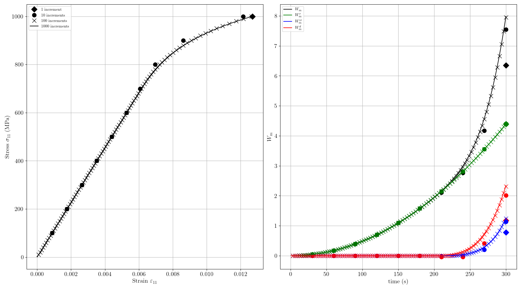
This example demonstrates the effect of increment size on the accuracy of the elastoplastic solver. We run the same loading path with increasing numbers of increments (1, 10, 100, 1000) and compare the stress-strain curves and energy terms. The elastic-plastic model with isotropic hardening (EPICP) is used as a representative case.

import os
import numpy as np
import matplotlib.pyplot as plt
import simcoon as sim

plt.rcParams["figure.figsize"] = (18, 10)

plt.rc("text", usetex=True)
plt.rc("font", family="serif")

# ###################################################################################
# Material definition
# --------------------
# We use an elastic-plastic material with isotropic hardening (EPICP):

umat_name = "EPICP"
nstatev = 8

E = 113800
nu = 0.342
alpha = 0.86e-5
sigma_Y = 600
H = 1600
beta = 0.25

psi_rve = 0.0
theta_rve = 0.0
phi_rve = 0.0
solver_type = 0
corate_type = 3

props = np.array([E, nu, alpha, sigma_Y, H, beta])
path_data = "../data"

# ###################################################################################
# Running the solver with different increment sizes
# ---------------------------------------------------
# We run 4 simulations with 1, 10, 100, and 1000 increments for the same
# loading path. With fewer increments, the implicit return-mapping algorithm
# takes larger steps, which can introduce errors in the plastic correction.

increments = [1, 10, 100, 1000]
data = []

for inc in increments:
    # Each path file is parsed in Python and its case runs in memory: nothing is
    # written to — or read back from — disk.
    pathfile = f"EPICP_path_{inc}.json"
    blocks, T_init, _ = sim.solver.load_path_json(os.path.join(path_data, pathfile))
    res = sim.solver.solve(
        blocks,
        umat_name,
        props,
        nstatev,
        T_init=T_init,
        solver_type=solver_type,
        corate=corate_type,
        orientation=(psi_rve, theta_rve, phi_rve),
    )
    Wm, Wm_r, Wm_ir, Wm_d = res["Wm"]
    data.append(
        {"e11": res["Strain"][0], "s11": res["Stress"][0], "time": res["Time"],
         "Wm": Wm, "Wm_r": Wm_r, "Wm_ir": Wm_ir, "Wm_d": Wm_d}
    )

# ###################################################################################
# Stress-strain convergence
# ---------------------------
# With only 1 increment, the solver jumps directly to the final state. As the
# number of increments increases, the stress-strain path converges to the
# reference solution (1000 increments).

fig, (ax1, ax2) = plt.subplots(1, 2)

markers = ["D", "o", "x", None]
labels = [f"{inc} increment{'s' if inc > 1 else ''}" for inc in increments]

ax1.grid(True)
ax1.tick_params(axis="both", which="major", labelsize=15)
ax1.set_xlabel(r"Strain $\varepsilon_{11}$", size=15)
ax1.set_ylabel(r"Stress $\sigma_{11}$ (MPa)", size=15)

for i, d in enumerate(data):
    if markers[i] is not None:
        ax1.plot(d["e11"], d["s11"], linestyle="None", marker=markers[i],
                 color="black", markersize=10, label=labels[i])
    else:
        ax1.plot(d["e11"], d["s11"], c="black", label=labels[i])
ax1.legend(loc="upper left")

# ###################################################################################
# Energy convergence
# --------------------
# The work terms should also converge. The mechanical work :math:`W_m` is
# decomposed into recoverable :math:`W_m^r`, irrecoverable :math:`W_m^{ir}`,
# and dissipated :math:`W_m^d` contributions.

ax2.grid(True)
ax2.tick_params(axis="both", which="major", labelsize=15)
ax2.set_xlabel("time (s)", size=15)
ax2.set_ylabel(r"$W_m$", size=15)

work_colors = ["black", "green", "blue", "red"]
work_keys = ["Wm", "Wm_r", "Wm_ir", "Wm_d"]
work_labels = [r"$W_m$", r"$W_m^r$", r"$W_m^{ir}$", r"$W_m^d$"]

for i, d in enumerate(data):
    for j, (wk, wc, wl) in enumerate(zip(work_keys, work_colors, work_labels)):
        label = wl if i == len(data) - 1 else None
        if markers[i] is not None:
            ax2.plot(d["time"], d[wk], linestyle="None", marker=markers[i],
                     color=wc, markersize=10, label=label)
        else:
            ax2.plot(d["time"], d[wk], c=wc, label=label)
ax2.legend(loc="upper left")

plt.tight_layout()
plt.show()