Micromechanics Examples

This example studies the evolution of the mechanical properties of a composite material considering spherical reinforcement.

import numpy as np
import matplotlib.pyplot as plt
from simcoon import simmit as sim
from simcoon import parameter as par
import os

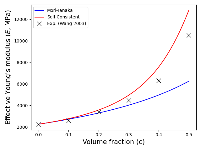
In this example we study the evolution of the mechanical properties of a 2-phase composite material considering spherical reinforcement. Two micromechanical schemes are utilized: Mori-Tanaka and Self-consistent.

First we define the number of state variables (if any) at the macroscopic level and the material properties.

dir = os.path.dirname(os.path.realpath("__file__"))
nstatev = 0

nphases = 2  # The number of phases
num_file = 0  # The num of the file that contains the subphases
int1 = 50
int2 = 50
n_matrix = 0

props = np.array([nphases, num_file, int1, int2, n_matrix], dtype="float")

There is a possibility to consider a misorientation between the test frame of reference and the composite material orientation, using Euler angles with the z–x–z convention. The stiffness tensor will be returned in the test frame of reference. We also specify which micromechanical scheme will be used:

• MIMTN → Mori-Tanaka scheme

• MISCN → Self-consistent scheme

path_data = dir + "/data"
path_keys = dir + "/keys"

param_list = par.read_parameters()

psi_rve = 0.0
theta_rve = 0.0
phi_rve = 0.0

Run the simulation to obtain the effective isotropic elastic properties for different volume fractions of reinforcement up to 50%.

concentration = np.arange(0.0, 0.51, 0.01)

E_MT = np.zeros(len(concentration))
umat_name = "MIMTN"
for i, x in enumerate(concentration):
    param_list[1].value = x
    param_list[0].value = 1.0 - x

    par.copy_parameters(param_list, path_keys, path_data)
    par.apply_parameters(param_list, path_data)

    L = sim.L_eff(umat_name, props, nstatev, psi_rve, theta_rve, phi_rve)
    p = sim.L_iso_props(L).flatten()
    E_MT[i] = p[0]


E_SC = np.zeros(len(concentration))
umat_name = "MISCN"
for i, x in enumerate(concentration):
    param_list[1].value = x
    param_list[0].value = 1.0 - x

    par.copy_parameters(param_list, path_keys, path_data)
    par.apply_parameters(param_list, path_data)

    L = sim.L_eff(umat_name, props, nstatev, psi_rve, theta_rve, phi_rve)
    p = sim.L_iso_props(L).flatten()
    E_SC[i] = p[0]

Plotting the results

In blue, we plot the effective Young’s modulus vs volume fraction curve using the Mori-Tanaka scheme, in red using the Self-Consistent scheme, and with black crosses the experimental data from (Wang 2003).

fig = plt.figure()
plt.xlabel(r"Volume fraction (c)", size=15)
plt.ylabel(r"Effective Young's modulus ($E$, MPa)", size=15)
plt.plot(concentration, E_MT, c="blue", label="Mori-Tanaka")
plt.plot(concentration, E_SC, c="red", label="Self-Consistent")
expfile = path_data + "/" + "E_exp.txt"
c, E = np.loadtxt(expfile, usecols=(0, 1), unpack=True)
plt.plot(
    c,
    E,
    linestyle="None",
    marker="x",
    color="black",
    markersize=10,
    label="Exp. (Wang 2003)",
)
plt.legend()
plt.tight_layout()
plt.show()

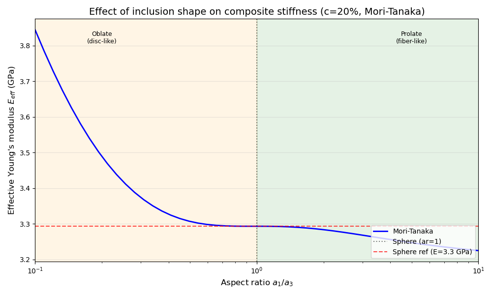
Effect of Aspect Ratio on Effective Stiffness

The shape of the reinforcement significantly affects the effective properties. Let’s study how the aspect ratio of prolate (fiber-like) and oblate (disc-like) inclusions influences the effective Young’s modulus using the Mori-Tanaka scheme.

The aspect ratio is defined as \(ar = a_1/a_3\), where:

• \(ar > 1\): prolate ellipsoid (fiber-like)

• \(ar = 1\): sphere

• \(ar < 1\): oblate ellipsoid (disc-like)

# Fixed volume fraction of 20%
c_reinf = 0.20
param_list[1].value = c_reinf
param_list[0].value = 1.0 - c_reinf
par.copy_parameters(param_list, path_keys, path_data)
par.apply_parameters(param_list, path_data)

# Aspect ratios from oblate (0.1) to prolate (10)
aspect_ratios = np.logspace(-1, 1, 50)

E_eff_ar = np.zeros(len(aspect_ratios))
umat_name = "MIMTN"

# Save original phase file
phase_file = path_data + "/Nellipsoids0.dat"
with open(phase_file, "r") as f:
    original_content = f.read()

print(f"\nComputing effective properties for c={c_reinf * 100:.0f}% reinforcement...")
for i, ar in enumerate(aspect_ratios):
    # Read and modify the phase file to set the aspect ratio
    with open(phase_file, "r") as f:
        lines = f.readlines()

    # Update semi-axes in reinforcement phase (line 2): a1/a3 = ar, a2 = a3 = 1
    parts = lines[2].split()
    parts[8] = str(ar)  # a1
    parts[9] = "1"  # a2
    parts[10] = "1"  # a3
    lines[2] = "\t".join(parts) + "\n"

    with open(phase_file, "w") as f:
        f.writelines(lines)

    L = sim.L_eff(umat_name, props, nstatev, psi_rve, theta_rve, phi_rve)
    p = sim.L_iso_props(L).flatten()
    E_eff_ar[i] = p[0]

# Restore original phase file
with open(phase_file, "w") as f:
    f.write(original_content)

# Get reference value for spherical inclusion (ar=1)
idx_sphere = np.argmin(np.abs(aspect_ratios - 1.0))
E_sphere_ref = E_eff_ar[idx_sphere]

Computing effective properties for c=20% reinforcement...

Plot: Effective Young’s modulus vs aspect ratio

This plot shows how inclusion shape dramatically affects composite stiffness. Prolate (fiber-like) inclusions are more effective at reinforcing the composite than oblate (disc-like) inclusions at the same volume fraction.

fig, ax = plt.subplots(figsize=(10, 6))
ax.semilogx(aspect_ratios, E_eff_ar / 1000, "b-", linewidth=2, label="Mori-Tanaka")
ax.axvline(x=1, color="k", linestyle=":", alpha=0.5, label="Sphere (ar=1)")
ax.axhline(
    y=E_sphere_ref / 1000,
    color="r",
    linestyle="--",
    alpha=0.7,
    label=f"Sphere ref (E={E_sphere_ref / 1000:.1f} GPa)",
)

# Add shaded regions for oblate/prolate
ymin, ymax = ax.get_ylim()
ax.axvspan(0.1, 1, alpha=0.1, color="orange")
ax.axvspan(1, 10, alpha=0.1, color="green")
ax.text(0.2, ymax - 0.1 * (ymax - ymin), "Oblate\n(disc-like)", fontsize=9, ha="center")
ax.text(5, ymax - 0.1 * (ymax - ymin), "Prolate\n(fiber-like)", fontsize=9, ha="center")

ax.set_xlabel("Aspect ratio $a_1/a_3$", fontsize=12)
ax.set_ylabel("Effective Young's modulus $E_{eff}$ (GPa)", fontsize=12)
ax.set_title(
    f"Effect of inclusion shape on composite stiffness (c={c_reinf * 100:.0f}%, Mori-Tanaka)",
    fontsize=14,
)
ax.legend(fontsize=10, loc="lower right")
ax.grid(True, alpha=0.3)
ax.set_xlim([0.1, 10])
plt.tight_layout()
plt.show()