Isotropic elasticity examples

import numpy as np
from simcoon import simmit as sim
import matplotlib.pyplot as plt
import os

In thermoelastic isotropic materials three parameters are required:

1. The Young modulus \(E\),

2. The Poisson ratio \(\nu\),

3. The coefficient of thermal expansion \(\alpha\).

The elastic stiffness tensor and the thermal expansion coefficients tensor are written in the Voigt notation formalism as

\[\begin{split}\mathbf{L} = \begin{pmatrix} L_{1111} & L_{1122} & L_{1122} & 0 & 0 & 0 \\ L_{1122} & L_{1111} & L_{1122} & 0 & 0 & 0 \\ L_{1122} & L_{1122} & L_{1111} & 0 & 0 & 0 \\ 0 & 0 & 0 & L_{1212} & 0 & 0 \\ 0 & 0 & 0 & 0 & L_{1212} & 0 \\ 0 & 0 & 0 & 0 & 0 & L_{1212} \end{pmatrix}, \quad \boldsymbol{\alpha} = \begin{pmatrix} \alpha & 0 & 0 \\ 0 & \alpha & 0 \\ 0 & 0 & \alpha \end{pmatrix}\end{split}\]

with

\[L_{1111} = \frac{E(1-\nu)}{(1+\nu)(1-2\nu)}, \quad L_{1122} = \frac{E\nu}{(1+\nu)(1-2\nu)}, \quad L_{1212} = \frac{E}{2(1+\nu)}.\]

The tangent stiffness tensor in this case is \(\mathbf{L}^t = \mathbf{L}\). Moreover, the increment of the elastic strain is given by

\[\Delta\varepsilon^{\mathrm{el}}_{ij} = \Delta\varepsilon^{\mathrm{tot}}_{ij} - \alpha \Delta T \delta_{ij},\]

where \(\delta_{ij}\) implies the Kronecker delta operator. In the 1D case only one component of stress is computed, through the relation

\[\sigma^{\mathrm{fin}}_{11} = \sigma^{\mathrm{init}}_{11} + E \Delta\varepsilon^{\mathrm{el}}_{11}.\]

In the plane stress case only three components of stress are computed, through the relations

\[\begin{split}\begin{pmatrix} \sigma^{\mathrm{fin}}_{11} \\ \sigma^{\mathrm{fin}}_{22} \\ \sigma^{\mathrm{fin}}_{12} \end{pmatrix} = \begin{pmatrix} \sigma^{\mathrm{init}}_{11} \\ \sigma^{\mathrm{init}}_{22} \\ \sigma^{\mathrm{init}}_{12} \end{pmatrix} + \frac{E}{1-\nu^2} \begin{pmatrix} 1 & \nu & 0 \\ \nu & 1 & 0 \\ 0 & 0 & \frac{1-\nu}{2} \end{pmatrix} \begin{pmatrix} \Delta\varepsilon^{\mathrm{el}}_{11} \\ \Delta\varepsilon^{\mathrm{el}}_{22} \\ 2\Delta\varepsilon^{\mathrm{el}}_{12} \end{pmatrix}\end{split}\]

In the generalized plane strain/3D analysis case the stress tensor is computed through the relation

\[\sigma^{\mathrm{fin}}_{ij} = \sigma^{\mathrm{init}}_{ij} + L_{ijkl}~\Delta\varepsilon^{\mathrm{el}}_{kl}.\]

umat_name = "ELISO"  # This is the 5 character code for the elastic-isotropic subroutine
nstatev = 1  # The number of scalar variables required, only the initial temperature is stored here

E = 700000.0
nu = 0.2
alpha = 1.0e-5

psi_rve = 0.0
theta_rve = 0.0
phi_rve = 0.0
solver_type = 0
corate_type = 2

props = np.array([E, nu, alpha])

path_data = "data"
path_results = "results"
pathfile = "ELISO_path.txt"
outputfile = "results_ELISO.txt"

sim.solver(
    umat_name,
    props,
    nstatev,
    psi_rve,
    theta_rve,
    phi_rve,
    solver_type,
    corate_type,
    path_data,
    path_results,
    pathfile,
    outputfile,
)

outputfile_macro = os.path.join(path_results, "results_ELISO_global-0.txt")

fig = plt.figure()

e11, e22, e33, e12, e13, e23, s11, s22, s33, s12, s13, s23 = np.loadtxt(
    outputfile_macro,
    usecols=(8, 9, 10, 11, 12, 13, 14, 15, 16, 17, 18, 19),
    unpack=True,
)

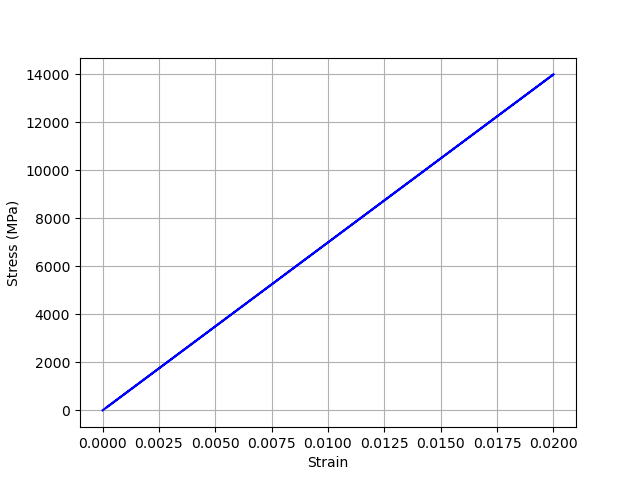
plt.grid(True)

plt.plot(e11, s11, c="blue")
plt.xlabel("Strain")
plt.ylabel("Stress (MPa)")

plt.show()