Yield Criteria Examples

This example demonstrates different yield criteria available in Simcoon, including von Mises, Tresca, Drucker, and anisotropic Hill criteria.

import numpy as np
from simcoon import simmit as sim
import matplotlib.pyplot as plt

Yield criteria are used to determine when a material begins to yield under a general stress state.

The general form of a yield criterion is:

\[\Phi(\boldsymbol{\sigma}) = \bar{\sigma} - \sigma_Y \leq 0\]

where \(\bar{\sigma}\) is the equivalent stress and \(\sigma_Y\) is the yield stress.

Von Mises equivalent stress

The von Mises equivalent stress is defined as:

\[\bar{\sigma}_{vM} = \sqrt{\frac{3}{2} \mathbf{s} : \mathbf{s}}\]

where \(\mathbf{s}\) is the deviatoric stress tensor.

# Define a uniaxial stress state in Voigt notation [s11, s22, s33, s12, s13, s23]
sigma_uniaxial = np.array([400.0, 0.0, 0.0, 0.0, 0.0, 0.0])

sigma_Mises = sim.Mises_stress(sigma_uniaxial)
print(f"Uniaxial stress: σ11 = {sigma_uniaxial[0]} MPa")
print(f"von Mises equivalent stress: {sigma_Mises:.2f} MPa")

# The von Mises stress equals the uniaxial stress for this case
print(
    f"Verification: σ_vM = σ11 for uniaxial tension ✓"
    if abs(sigma_Mises - 400) < 1e-6
    else ""
)

Uniaxial stress: σ11 = 400.0 MPa
von Mises equivalent stress: 400.00 MPa
Verification: σ_vM = σ11 for uniaxial tension ✓

Tresca equivalent stress

The Tresca criterion is based on the maximum shear stress:

\[\bar{\sigma}_{T} = \sigma_1 - \sigma_3\]

where \(\sigma_1\) and \(\sigma_3\) are the maximum and minimum principal stresses.

sigma_Tresca = sim.Tresca_stress(sigma_uniaxial)
print(f"\nTresca equivalent stress: {sigma_Tresca:.2f} MPa")
print("For uniaxial tension, Tresca = von Mises = σ11")

# Compute the gradient (flow direction)
dsigma_Tresca = sim.dTresca_stress(sigma_uniaxial)
print(f"Tresca flow direction: {np.array_str(dsigma_Tresca, precision=4)}")

Tresca equivalent stress: 400.00 MPa
For uniaxial tension, Tresca = von Mises = σ11
Tresca flow direction: [[ 1. ]
 [-0.5]
 [-0.5]
 [ 0. ]
 [ 0. ]
 [ 0. ]]

Drucker equivalent stress

The Drucker criterion generalizes the von Mises criterion:

\[\bar{\sigma}_{D} = \left[ (J_2)^3 - b (J_3)^2 \right]^{1/n}\]

where \(J_2\) and \(J_3\) are the second and third invariants of the deviatoric stress, \(b\) is a material parameter, and \(n\) is an exponent.

b = 0.0  # When b=0 and n=2, Drucker reduces to von Mises
n = 2.0
props_Drucker = np.array([b, n])

sigma_Drucker = sim.Drucker_stress(sigma_uniaxial, props_Drucker)
print(f"\nDrucker equivalent stress (b={b}, n={n}): {sigma_Drucker:.2f} MPa")
print("With b=0 and n=2, Drucker ≈ von Mises")

# Compute the gradient
dsigma_Drucker = sim.dDrucker_stress(sigma_uniaxial, props_Drucker)
print(f"Drucker flow direction: {np.array_str(dsigma_Drucker, precision=4)}")

Drucker equivalent stress (b=0.0, n=2.0): 400.00 MPa
With b=0 and n=2, Drucker ≈ von Mises
Drucker flow direction: [[ 1. ]
 [-0.5]
 [-0.5]
 [ 0. ]
 [ 0. ]
 [ 0. ]]

Hill anisotropic yield criterion

The Hill criterion extends von Mises to orthotropic materials:

\[\bar{\sigma}_{H}^2 = F(\sigma_{22}-\sigma_{33})^2 + G(\sigma_{33}-\sigma_{11})^2 + H(\sigma_{11}-\sigma_{22})^2 + 2L\sigma_{23}^2 + 2M\sigma_{13}^2 + 2N\sigma_{12}^2\]

For isotropic materials: F = G = H = 0.5 and L = M = N = 1.5

# Isotropic Hill parameters (equivalent to von Mises)
F, G, H = 0.5, 0.5, 0.5
L, M, N = 1.5, 1.5, 1.5
props_Hill = np.array([F, G, H, L, M, N])

sigma_Hill = sim.Hill_stress(sigma_uniaxial, props_Hill)
print(f"\nHill equivalent stress (isotropic params): {sigma_Hill:.2f} MPa")
print("With isotropic parameters, Hill = von Mises")

# Anisotropic case: material is stronger in direction 1
F_aniso, G_aniso, H_aniso = 0.3, 0.6, 0.6  # Lower F means σ22-σ33 matters less
L_aniso, M_aniso, N_aniso = 1.5, 1.5, 1.5
props_Hill_aniso = np.array([F_aniso, G_aniso, H_aniso, L_aniso, M_aniso, N_aniso])

sigma_Hill_aniso = sim.Hill_stress(sigma_uniaxial, props_Hill_aniso)
print(f"Hill equivalent stress (anisotropic): {sigma_Hill_aniso:.2f} MPa")

Hill equivalent stress (isotropic params): 400.00 MPa
With isotropic parameters, Hill = von Mises
Hill equivalent stress (anisotropic): 438.18 MPa

Hill configurational tensor

The Hill criterion can be written in matrix form:

\[\bar{\sigma}_{H}^2 = \boldsymbol{\sigma}^T \mathbf{P} \boldsymbol{\sigma}\]

where \(\mathbf{P}\) is the Hill configurational tensor.

P_Hill = sim.P_Hill(props_Hill)
print("\nHill configurational tensor P (isotropic):")
print(np.array_str(P_Hill, precision=4, suppress_small=True))

Hill configurational tensor P (isotropic):
[[ 1.  -0.5 -0.5  0.   0.   0. ]
 [-0.5  1.  -0.5  0.   0.   0. ]
 [-0.5 -0.5  1.   0.   0.   0. ]
 [ 0.   0.   0.   3.   0.   0. ]
 [ 0.   0.   0.   0.   3.   0. ]
 [ 0.   0.   0.   0.   0.   3. ]]

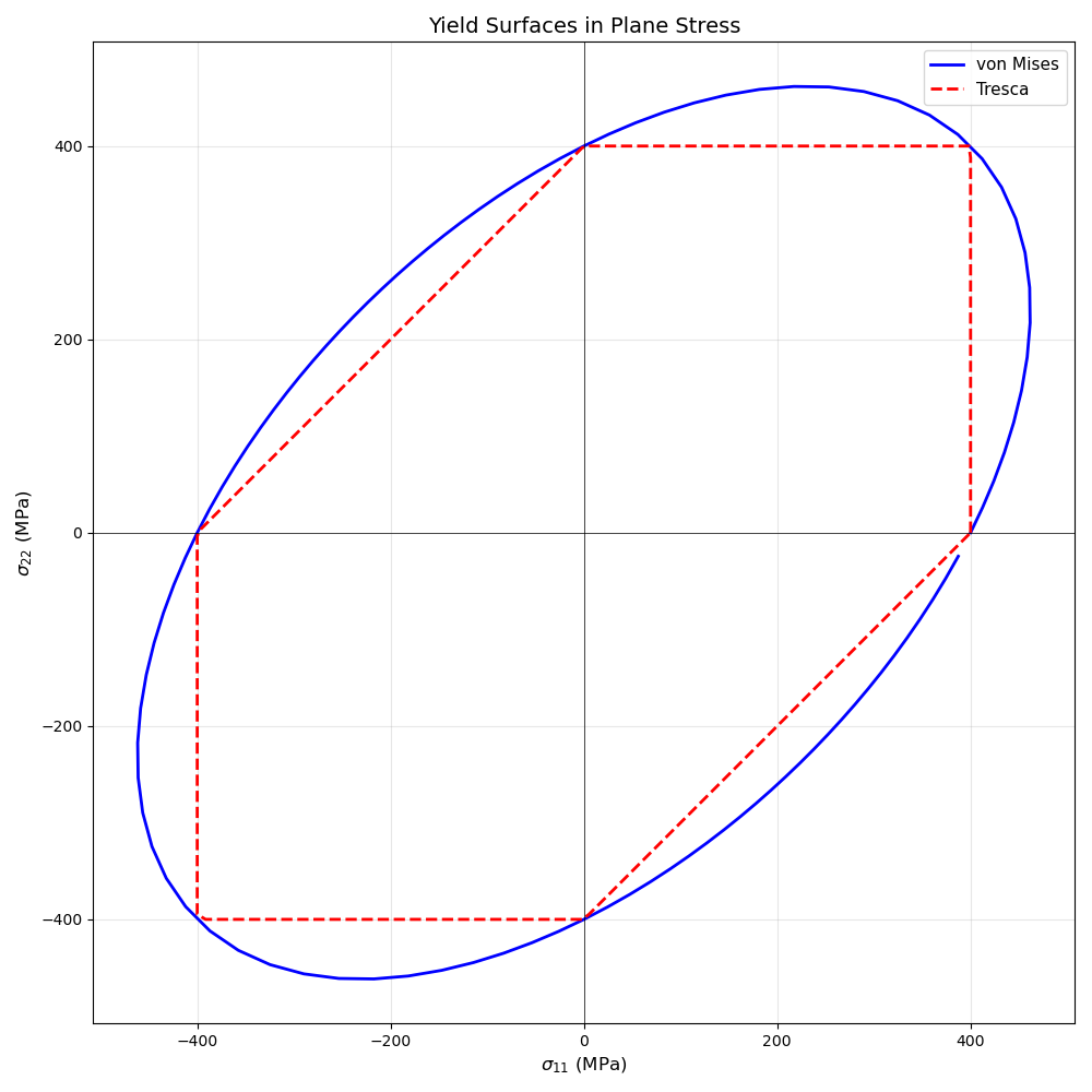
Yield surface visualization

Let’s visualize the yield surfaces in the σ11-σ22 plane (plane stress).

theta = np.linspace(0, 2 * np.pi, 360)
sigma_Y = 400.0  # Yield stress

# von Mises yield surface (ellipse in principal stress space)
s11_vM = sigma_Y * np.cos(theta)
s22_vM = sigma_Y * (np.cos(theta) * 0.5 + np.sin(theta) * np.sqrt(3) / 2)

# Tresca yield surface (hexagon)
# Computing Tresca surface points
s11_T = []
s22_T = []
for t in theta:
    # Sample stress states on a circle and find where Tresca = sigma_Y
    s11 = sigma_Y * np.cos(t)
    s22 = sigma_Y * np.sin(t)
    sigma_test = np.array([s11, s22, 0.0, 0.0, 0.0, 0.0])
    sig_T = sim.Tresca_stress(sigma_test)
    if sig_T > 1e-6:
        scale = sigma_Y / sig_T
        s11_T.append(s11 * scale)
        s22_T.append(s22 * scale)

fig, ax = plt.subplots(figsize=(10, 10))

# Plot von Mises (approximated as ellipse)
n_points = 100
s11_plot = []
s22_plot = []
for i in range(n_points):
    t = 2 * np.pi * i / n_points
    s11 = 1.2 * sigma_Y * np.cos(t)
    s22 = 1.2 * sigma_Y * np.sin(t)
    sigma_test = np.array([s11, s22, 0.0, 0.0, 0.0, 0.0])
    sig_vM = sim.Mises_stress(sigma_test)
    if sig_vM > 1e-6:
        scale = sigma_Y / sig_vM
        s11_plot.append(s11 * scale)
        s22_plot.append(s22 * scale)

ax.plot(s11_plot, s22_plot, "b-", linewidth=2, label="von Mises")
ax.plot(s11_T, s22_T, "r--", linewidth=2, label="Tresca")

ax.set_xlabel(r"$\sigma_{11}$ (MPa)", fontsize=12)
ax.set_ylabel(r"$\sigma_{22}$ (MPa)", fontsize=12)
ax.set_title("Yield Surfaces in Plane Stress", fontsize=14)
ax.legend(fontsize=11)
ax.set_aspect("equal")
ax.grid(True, alpha=0.3)
ax.axhline(y=0, color="k", linewidth=0.5)
ax.axvline(x=0, color="k", linewidth=0.5)
plt.tight_layout()
plt.show()

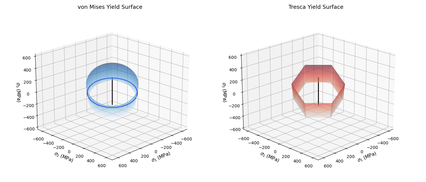
3D Yield Surfaces

The yield surfaces can be visualized in 3D principal stress space \((\sigma_1, \sigma_2, \sigma_3)\). In this space:

• The hydrostatic axis is the line \(\sigma_1 = \sigma_2 = \sigma_3\)

• Deviatoric planes are perpendicular to the hydrostatic axis

• von Mises surface is a cylinder along the hydrostatic axis

• Tresca surface is a hexagonal prism along the hydrostatic axis

We’ll visualize cross-sections at constant hydrostatic pressure (π-planes).

from mpl_toolkits.mplot3d import Axes3D
from matplotlib import cm, colors

The von Mises criterion is independent of hydrostatic stress, forming a cylinder of radius \(\sqrt{2/3} \sigma_Y\) around the hydrostatic axis.

# Create a parametric cylinder along the hydrostatic axis
n_theta = 60
n_z = 20
theta_3d = np.linspace(0, 2 * np.pi, n_theta)
z_hydro = np.linspace(-1.5 * sigma_Y, 1.5 * sigma_Y, n_z)

# The hydrostatic axis direction (1,1,1)/sqrt(3)
# Perpendicular directions in deviatoric plane
e_hydro = np.array([1, 1, 1]) / np.sqrt(3)
e1_dev = np.array([1, -1, 0]) / np.sqrt(2)
e2_dev = np.array([1, 1, -2]) / np.sqrt(6)

# von Mises radius in deviatoric plane
r_vM = np.sqrt(2 / 3) * sigma_Y

# Generate surface points
Theta, Z = np.meshgrid(theta_3d, z_hydro)
S1_vM = np.zeros_like(Theta)
S2_vM = np.zeros_like(Theta)
S3_vM = np.zeros_like(Theta)

for i in range(n_z):
    for j in range(n_theta):
        # Point on cylinder
        p = (
            z_hydro[i] * e_hydro
            + r_vM * np.cos(theta_3d[j]) * e1_dev
            + r_vM * np.sin(theta_3d[j]) * e2_dev
        )
        S1_vM[i, j] = p[0]
        S2_vM[i, j] = p[1]
        S3_vM[i, j] = p[2]

The Tresca criterion forms a hexagonal prism inscribed within the von Mises cylinder. The hexagon vertices touch the von Mises cylinder.

# Generate Tresca hexagonal prism
n_hex = 7  # 6 sides + close the loop

# Hexagon vertices at angles 0, 60, 120, 180, 240, 300 degrees
hex_angles = np.linspace(0, 2 * np.pi, n_hex)
# Tresca radius varies around the deviatoric plane - hexagon inscribed in circle
# At vertices: r = r_vM, at edges: r = r_vM * cos(30°)

S1_T_list = []
S2_T_list = []
S3_T_list = []

for i in range(n_z):
    s1_row = []
    s2_row = []
    s3_row = []
    for j in range(n_hex):
        # Tresca forms a hexagon - scale to touch von Mises at vertices
        angle = hex_angles[j]
        # Tresca inscribed in von Mises cylinder
        r_T = r_vM * 2 / np.sqrt(3) * np.cos(np.pi / 6 - np.mod(angle, np.pi / 3))
        p = (
            z_hydro[i] * e_hydro
            + r_T * np.cos(angle) * e1_dev
            + r_T * np.sin(angle) * e2_dev
        )
        s1_row.append(p[0])
        s2_row.append(p[1])
        s3_row.append(p[2])
    S1_T_list.append(s1_row)
    S2_T_list.append(s2_row)
    S3_T_list.append(s3_row)

S1_T_3d = np.array(S1_T_list)
S2_T_3d = np.array(S2_T_list)
S3_T_3d = np.array(S3_T_list)

Interactive 3D visualization showing von Mises (cylinder) and Tresca (hexagonal prism) yield surfaces along with the hydrostatic axis.

fig = plt.figure(figsize=(14, 6))

# Left subplot: von Mises surface
ax1 = fig.add_subplot(121, projection="3d")
ax1.plot_surface(
    S1_vM, S2_vM, S3_vM, alpha=0.6, cmap=cm.Blues, edgecolor="none", shade=True
)
# Add hydrostatic axis
t_axis = np.linspace(-1.5 * sigma_Y, 1.5 * sigma_Y, 50)
ax1.plot(t_axis, t_axis, t_axis, "k-", linewidth=2, label="Hydrostatic axis")
# Add deviatoric plane at σ_m = 0
ax1.plot(s11_plot, s22_plot, [0] * len(s11_plot), "b-", linewidth=2)
ax1.set_xlabel(r"$\sigma_1$ (MPa)", fontsize=11)
ax1.set_ylabel(r"$\sigma_2$ (MPa)", fontsize=11)
ax1.set_zlabel(r"$\sigma_3$ (MPa)", fontsize=11)
ax1.set_title("von Mises Yield Surface", fontsize=13)
ax1.view_init(elev=20, azim=45)

# Right subplot: Tresca surface
ax2 = fig.add_subplot(122, projection="3d")
ax2.plot_surface(
    S1_T_3d, S2_T_3d, S3_T_3d, alpha=0.6, cmap=cm.Reds, edgecolor="gray", linewidth=0.3
)
# Add hydrostatic axis
ax2.plot(t_axis, t_axis, t_axis, "k-", linewidth=2, label="Hydrostatic axis")
ax2.set_xlabel(r"$\sigma_1$ (MPa)", fontsize=11)
ax2.set_ylabel(r"$\sigma_2$ (MPa)", fontsize=11)
ax2.set_zlabel(r"$\sigma_3$ (MPa)", fontsize=11)
ax2.set_title("Tresca Yield Surface", fontsize=13)
ax2.view_init(elev=20, azim=45)

plt.tight_layout()
plt.show()

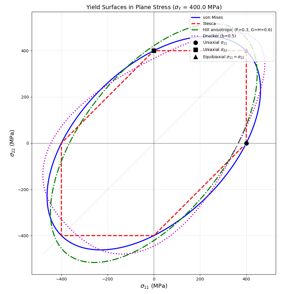
Plane Stress (σ₁₁, σ₂₂)

In plane stress conditions (\(\sigma_{33} = \sigma_{13} = \sigma_{23} = 0\)), yield surfaces can be visualized in the \((\sigma_{11}, \sigma_{22})\) plane. This is the classical representation for comparing yield criteria.

n_points_surf = 200
theta_surf = np.linspace(0, 2 * np.pi, n_points_surf)


# Generate yield surface points for each criterion
def compute_yield_surface_s11_s22(criterion_func, props=None, n_pts=200):
    """Compute yield surface in (σ11, σ22) plane stress space."""
    s11_list = []
    s22_list = []
    for i in range(n_pts):
        t = 2 * np.pi * i / n_pts
        # Sample on a circle larger than yield surface
        s11 = 1.5 * sigma_Y * np.cos(t)
        s22 = 1.5 * sigma_Y * np.sin(t)
        sigma_test = np.array([s11, s22, 0.0, 0.0, 0.0, 0.0])
        if props is not None:
            sig_eq = criterion_func(sigma_test, props)
        else:
            sig_eq = criterion_func(sigma_test)
        if sig_eq > 1e-6:
            scale = sigma_Y / sig_eq
            s11_list.append(s11 * scale)
            s22_list.append(s22 * scale)
    return s11_list, s22_list


# von Mises
s11_vM, s22_vM = compute_yield_surface_s11_s22(sim.Mises_stress)

# Tresca
s11_Tr, s22_Tr = compute_yield_surface_s11_s22(sim.Tresca_stress)

# Hill isotropic (should match von Mises)
s11_Hill_iso, s22_Hill_iso = compute_yield_surface_s11_s22(sim.Hill_stress, props_Hill)

# Hill anisotropic
s11_Hill_aniso, s22_Hill_aniso = compute_yield_surface_s11_s22(
    sim.Hill_stress, props_Hill_aniso
)

# Drucker with b=0.5
props_Drucker_plane = np.array([0.5, 2.0])
s11_Drucker, s22_Drucker = compute_yield_surface_s11_s22(
    sim.Drucker_stress, props_Drucker_plane
)

fig, ax = plt.subplots(figsize=(10, 10))

ax.plot(s11_vM, s22_vM, "b-", linewidth=2.5, label="von Mises")
ax.plot(s11_Tr, s22_Tr, "r--", linewidth=2.5, label="Tresca")
ax.plot(
    s11_Hill_aniso,
    s22_Hill_aniso,
    "g-.",
    linewidth=2.5,
    label="Hill anisotropic (F=0.3, G=H=0.6)",
)
ax.plot(s11_Drucker, s22_Drucker, "m:", linewidth=2.5, label="Drucker (b=0.5)")

# Add key stress states
ax.plot(sigma_Y, 0, "ko", markersize=10, label=r"Uniaxial $\sigma_{11}$")
ax.plot(0, sigma_Y, "ks", markersize=10, label=r"Uniaxial $\sigma_{22}$")
ax.plot(
    sigma_Y,
    sigma_Y,
    "k^",
    markersize=10,
    label=r"Equibiaxial $\sigma_{11}=\sigma_{22}$",
)

ax.set_xlabel(r"$\sigma_{11}$ (MPa)", fontsize=14)
ax.set_ylabel(r"$\sigma_{22}$ (MPa)", fontsize=14)
ax.set_title(
    f"Yield Surfaces in Plane Stress ($\\sigma_Y$ = {sigma_Y} MPa)", fontsize=14
)
ax.legend(fontsize=10, loc="upper right")
ax.set_aspect("equal")
ax.grid(True, alpha=0.3)
ax.axhline(y=0, color="k", linewidth=0.5)
ax.axvline(x=0, color="k", linewidth=0.5)

# Add diagonal for equibiaxial loading
ax.plot(
    [-sigma_Y * 1.2, sigma_Y * 1.2],
    [-sigma_Y * 1.2, sigma_Y * 1.2],
    "k:",
    alpha=0.3,
    linewidth=1,
)

plt.tight_layout()
plt.show()

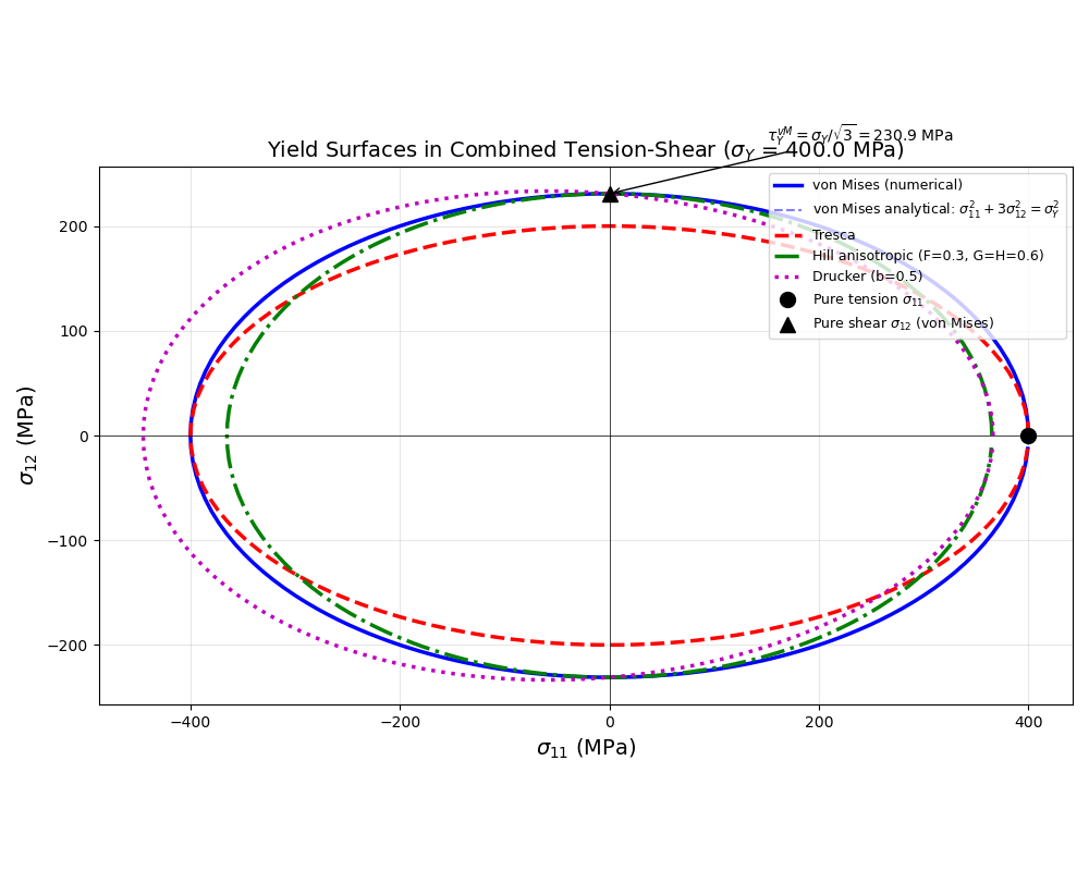
Tension-Shear (σ₁₁, σ₁₂)

Another important representation is the combined tension-shear space \((\sigma_{11}, \sigma_{12})\), which is relevant for many practical loading conditions.

For von Mises under combined tension and shear:

\[\sigma_{11}^2 + 3\sigma_{12}^2 = \sigma_Y^2\]

def compute_yield_surface_s11_s12(criterion_func, props=None, n_pts=200):
    """Compute yield surface in (σ11, σ12) combined stress space."""
    s11_list = []
    s12_list = []
    for i in range(n_pts):
        t = 2 * np.pi * i / n_pts
        # Sample on a circle larger than yield surface
        s11 = 1.5 * sigma_Y * np.cos(t)
        s12 = 1.5 * sigma_Y * np.sin(t)
        # Plane stress with shear: σ = [σ11, σ22, σ33, σ12, σ13, σ23]
        sigma_test = np.array([s11, 0.0, 0.0, s12, 0.0, 0.0])
        if props is not None:
            sig_eq = criterion_func(sigma_test, props)
        else:
            sig_eq = criterion_func(sigma_test)
        if sig_eq > 1e-6:
            scale = sigma_Y / sig_eq
            s11_list.append(s11 * scale)
            s12_list.append(s12 * scale)
    return s11_list, s12_list


# von Mises
s11_vM_shear, s12_vM = compute_yield_surface_s11_s12(sim.Mises_stress)

# Tresca
s11_Tr_shear, s12_Tr = compute_yield_surface_s11_s12(sim.Tresca_stress)

# Hill anisotropic
s11_Hill_shear, s12_Hill = compute_yield_surface_s11_s12(
    sim.Hill_stress, props_Hill_aniso
)

# Drucker
s11_Drucker_shear, s12_Drucker = compute_yield_surface_s11_s12(
    sim.Drucker_stress, props_Drucker_plane
)

# Analytical von Mises ellipse for reference: σ11² + 3σ12² = σY²
theta_ana = np.linspace(0, 2 * np.pi, 200)
s11_vM_ana = sigma_Y * np.cos(theta_ana)
s12_vM_ana = sigma_Y / np.sqrt(3) * np.sin(theta_ana)

fig, ax = plt.subplots(figsize=(10, 8))

ax.plot(s11_vM_shear, s12_vM, "b-", linewidth=2.5, label="von Mises (numerical)")
ax.plot(
    s11_vM_ana,
    s12_vM_ana,
    "b--",
    linewidth=1.5,
    alpha=0.5,
    label=r"von Mises analytical: $\sigma_{11}^2 + 3\sigma_{12}^2 = \sigma_Y^2$",
)
ax.plot(s11_Tr_shear, s12_Tr, "r--", linewidth=2.5, label="Tresca")
ax.plot(
    s11_Hill_shear,
    s12_Hill,
    "g-.",
    linewidth=2.5,
    label="Hill anisotropic (F=0.3, G=H=0.6)",
)
ax.plot(s11_Drucker_shear, s12_Drucker, "m:", linewidth=2.5, label="Drucker (b=0.5)")

# Add key stress states
ax.plot(sigma_Y, 0, "ko", markersize=10, label=r"Pure tension $\sigma_{11}$")
ax.plot(
    0,
    sigma_Y / np.sqrt(3),
    "k^",
    markersize=10,
    label=r"Pure shear $\sigma_{12}$ (von Mises)",
)

ax.set_xlabel(r"$\sigma_{11}$ (MPa)", fontsize=14)
ax.set_ylabel(r"$\sigma_{12}$ (MPa)", fontsize=14)
ax.set_title(
    f"Yield Surfaces in Combined Tension-Shear ($\\sigma_Y$ = {sigma_Y} MPa)",
    fontsize=14,
)
ax.legend(fontsize=9, loc="upper right")
ax.set_aspect("equal")
ax.grid(True, alpha=0.3)
ax.axhline(y=0, color="k", linewidth=0.5)
ax.axvline(x=0, color="k", linewidth=0.5)

# Add yield stress in pure shear annotation
tau_Y_vM = sigma_Y / np.sqrt(3)
ax.annotate(
    rf"$\tau_Y^{{vM}} = \sigma_Y/\sqrt{{3}} = {tau_Y_vM:.1f}$ MPa",
    xy=(0, tau_Y_vM),
    xytext=(150, tau_Y_vM + 50),
    fontsize=10,
    arrowprops=dict(arrowstyle="->", color="black"),
)

plt.tight_layout()
plt.show()

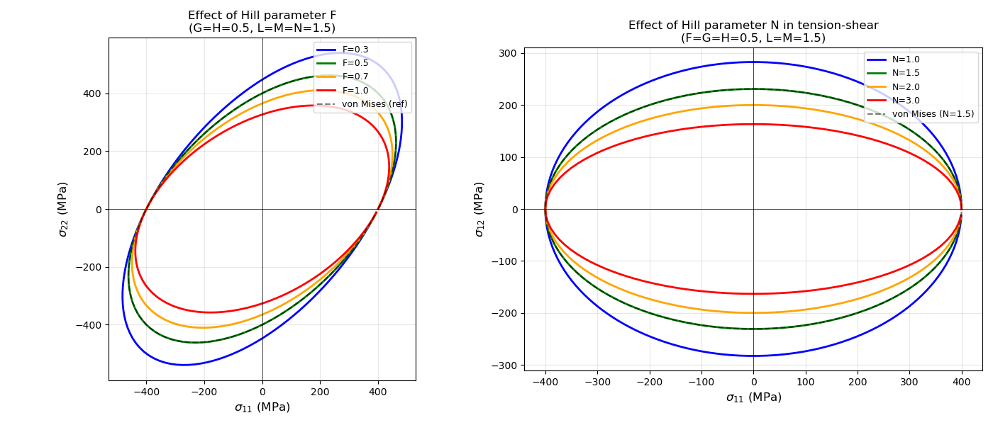
Hill Anisotropy Parameters

The Hill criterion captures anisotropic yielding. Let’s see how different parameters affect the yield surface in the \((\sigma_{11}, \sigma_{22})\) plane.

fig, axes = plt.subplots(1, 2, figsize=(14, 6))

# Left plot: Effect of F parameter (keeping G=H=0.5, L=M=N=1.5)
ax = axes[0]
F_values = [0.3, 0.5, 0.7, 1.0]
colors_F = ["blue", "green", "orange", "red"]

for F_val, col in zip(F_values, colors_F):
    props_test = np.array([F_val, 0.5, 0.5, 1.5, 1.5, 1.5])
    s11_test, s22_test = compute_yield_surface_s11_s22(sim.Hill_stress, props_test)
    ax.plot(s11_test, s22_test, "-", linewidth=2, color=col, label=f"F={F_val}")

ax.plot(s11_vM, s22_vM, "k--", linewidth=1.5, alpha=0.5, label="von Mises (ref)")
ax.set_xlabel(r"$\sigma_{11}$ (MPa)", fontsize=12)
ax.set_ylabel(r"$\sigma_{22}$ (MPa)", fontsize=12)
ax.set_title("Effect of Hill parameter F\n(G=H=0.5, L=M=N=1.5)", fontsize=12)
ax.legend(fontsize=9, loc="upper right")
ax.set_aspect("equal")
ax.grid(True, alpha=0.3)
ax.axhline(y=0, color="k", linewidth=0.5)
ax.axvline(x=0, color="k", linewidth=0.5)

# Right plot: Effect of N parameter (keeping F=G=H=0.5, L=M=1.5)
# N controls the σ₁₂ shear contribution in Hill criterion
# For tension-shear (σ₁₁, σ₁₂), we vary N to see its effect
ax = axes[1]
N_values = [1.0, 1.5, 2.0, 3.0]
colors_N = ["blue", "green", "orange", "red"]


for N_val, col in zip(N_values, colors_N):
    props_test = np.array([0.5, 0.5, 0.5, 1.5, 1.5, N_val])
    s11_test, s12_test = compute_yield_surface_s11_s12(sim.Hill_stress, props_test)
    ax.plot(s11_test, s12_test, "-", linewidth=2, color=col, label=f"N={N_val}")

# Reference: von Mises analytical ellipse
ax.plot(
    s11_vM_ana, s12_vM_ana, "k--", linewidth=1.5, alpha=0.5, label="von Mises (N=1.5)"
)
ax.set_xlabel(r"$\sigma_{11}$ (MPa)", fontsize=12)
ax.set_ylabel(r"$\sigma_{12}$ (MPa)", fontsize=12)
ax.set_title(
    "Effect of Hill parameter N in tension-shear\n(F=G=H=0.5, L=M=1.5)", fontsize=12
)
ax.legend(fontsize=9, loc="upper right")
ax.set_aspect("equal")
ax.grid(True, alpha=0.3)
ax.axhline(y=0, color="k", linewidth=0.5)
ax.axvline(x=0, color="k", linewidth=0.5)

plt.tight_layout()
plt.show()

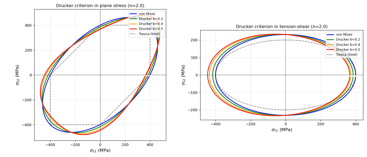
Drucker Parameter b

The Drucker criterion with parameter \(b\) and exponent \(n\) generalizes von Mises. Let’s visualize this in both stress spaces. Valid range for b is approximately \(-0.27 \leq b \leq 0.5\) for convexity.

b_values = [0.0, 0.2, 0.4, 0.5]
n_exp = 2.0
colors_b = ["blue", "green", "orange", "red"]

fig, axes = plt.subplots(1, 2, figsize=(14, 6))

# Left: (σ11, σ22) plane
ax = axes[0]
for b_val, col in zip(b_values, colors_b):
    props_D = np.array([b_val, n_exp])
    s11_D, s22_D = compute_yield_surface_s11_s22(sim.Drucker_stress, props_D)
    label = "von Mises" if b_val == 0 else f"Drucker b={b_val}"
    ax.plot(s11_D, s22_D, "-", linewidth=2, color=col, label=label)

ax.plot(s11_Tr, s22_Tr, "k--", linewidth=1.5, alpha=0.5, label="Tresca (limit)")
ax.set_xlabel(r"$\sigma_{11}$ (MPa)", fontsize=12)
ax.set_ylabel(r"$\sigma_{22}$ (MPa)", fontsize=12)
ax.set_title(f"Drucker criterion in plane stress (n={n_exp})", fontsize=12)
ax.legend(fontsize=9, loc="upper right")
ax.set_aspect("equal")
ax.grid(True, alpha=0.3)
ax.axhline(y=0, color="k", linewidth=0.5)
ax.axvline(x=0, color="k", linewidth=0.5)

# Right: (σ11, σ12) plane
ax = axes[1]
for b_val, col in zip(b_values, colors_b):
    props_D = np.array([b_val, n_exp])
    s11_D, s12_D = compute_yield_surface_s11_s12(sim.Drucker_stress, props_D)
    label = "von Mises" if b_val == 0 else f"Drucker b={b_val}"
    ax.plot(s11_D, s12_D, "-", linewidth=2, color=col, label=label)

ax.plot(s11_Tr_shear, s12_Tr, "k--", linewidth=1.5, alpha=0.5, label="Tresca (limit)")
ax.set_xlabel(r"$\sigma_{11}$ (MPa)", fontsize=12)
ax.set_ylabel(r"$\sigma_{12}$ (MPa)", fontsize=12)
ax.set_title(f"Drucker criterion in tension-shear (n={n_exp})", fontsize=12)
ax.legend(fontsize=9, loc="upper right")
ax.set_aspect("equal")
ax.grid(True, alpha=0.3)
ax.axhline(y=0, color="k", linewidth=0.5)
ax.axvline(x=0, color="k", linewidth=0.5)

plt.tight_layout()
plt.show()