Prony Series Viscoelastic Model (Generalized Maxwell)

import numpy as np
import matplotlib.pyplot as plt
import simcoon as sim
import os

plt.rcParams["figure.figsize"] = (18, 10)

The Prony series (generalized Maxwell) constitutive law is a rate-dependent, isotropic, linear viscoelastic model that considers thermal strains. It extends the Zener (standard linear solid) model to \(N\) Maxwell branches connected in parallel with a long-term elastic spring.

The material parameters are:

1. The long-term (equilibrium) Young’s modulus \(E_0\)

2. The long-term Poisson’s ratio \(\nu_0\)

3. The coefficient of thermal expansion \(\alpha\)

4. The number of Prony branches \(N\)

Then, for each branch \(i = 1, \ldots, N\):

5. The branch Young’s modulus \(E_i\)

6. The branch Poisson’s ratio \(\nu_i\)

7. The branch bulk viscosity \(\eta_{B,i}\)

8. The branch shear viscosity \(\eta_{S,i}\)

The constitutive law is given by:

\[\boldsymbol{\sigma}(t) = \mathbf{L}_0 : \boldsymbol{\varepsilon}(t) + \sum_{i=1}^{N} \mathbf{L}_i : \boldsymbol{\varepsilon}^{v}_i(t)\]

where each viscous strain \(\boldsymbol{\varepsilon}^{v}_i\) evolves according to the Maxwell element ODE with characteristic viscosities \(\eta_{B,i}\) and \(\eta_{S,i}\).

umat_name = "PRONK"  # 5 character code for the generalized Maxwell (Prony) model

E_0 = 9400.0  # Long-term Young's modulus (MPa)
nu_0 = 0.4  # Long-term Poisson's ratio
alpha = 0.0  # Coefficient of thermal expansion
n_prony = 5  # Number of Prony (Maxwell) branches

# Read branch parameters from data file
path_data = "../data"
mat_file = os.path.join(path_data, "Prony_raw.dat")
E_i, nu_i, etaB_i, etaS_i = np.loadtxt(mat_file, usecols=(0, 1, 2, 3), unpack=True)

# nstatev depends on the number of branches
nstatev = 8 + 7 * n_prony  # Number of internal state variables

psi_rve = 0.0
theta_rve = 0.0
phi_rve = 0.0
solver_type = 0
corate_type = 1

# Build the properties array: [E_0, nu_0, alpha, n_prony, E_1, nu_1, etaB_1, etaS_1, ...]
props = np.array([E_0, nu_0, alpha, n_prony])
for i in range(n_prony):
    props = np.append(props, [E_i[i], nu_i[i], etaB_i[i], etaS_i[i]])

path_results = "results"
pathfile = "PRONK_path.txt"
outputfile = "results_PRONK.txt"

sim.solver(
    umat_name,
    props,
    nstatev,
    psi_rve,
    theta_rve,
    phi_rve,
    solver_type,
    corate_type,
    path_data,
    path_results,
    pathfile,
    outputfile,
)

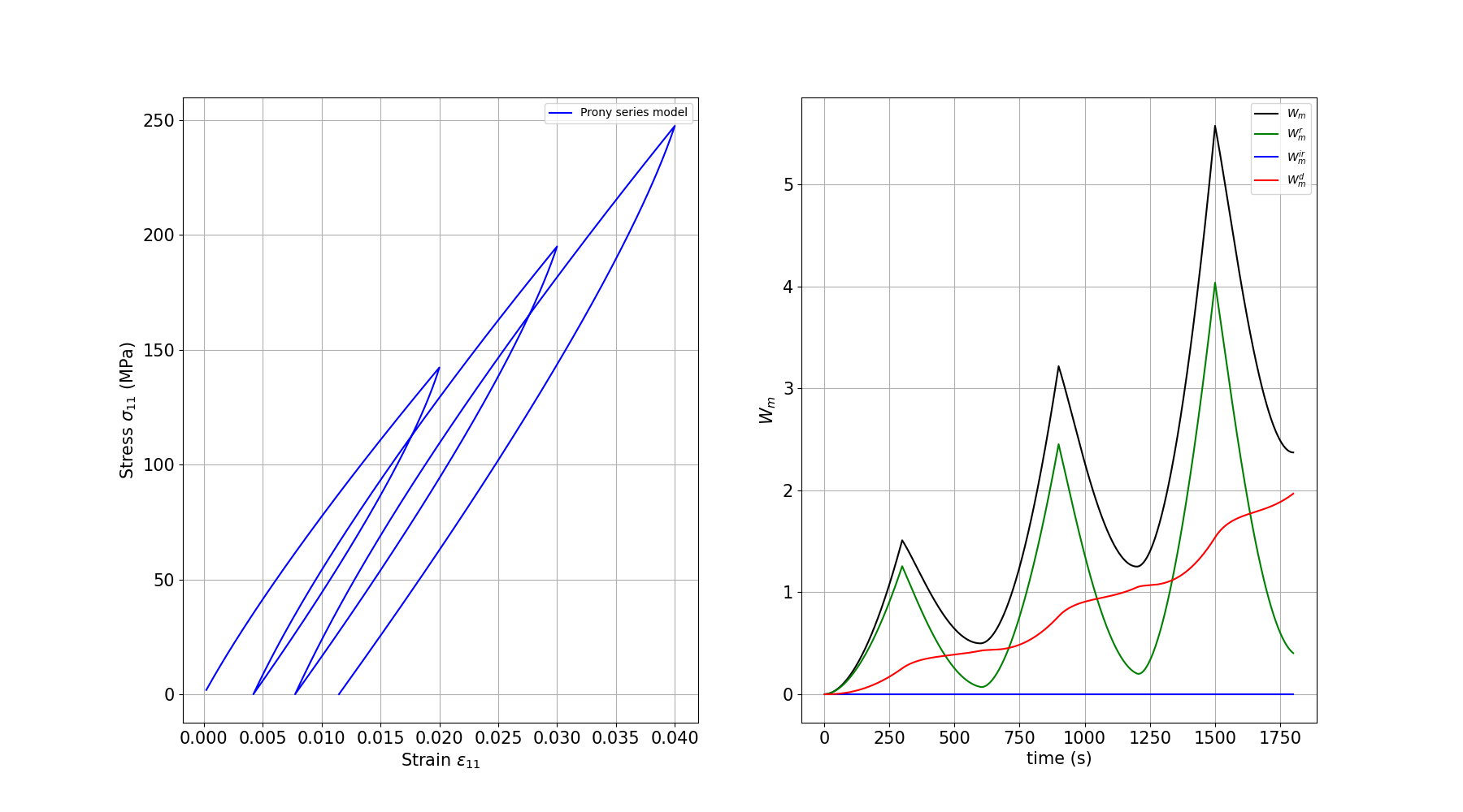
Plotting the results

We plot the stress-strain response which shows the viscoelastic behavior (rate-dependent stiffness and hysteresis from viscous dissipation).

outputfile_macro = os.path.join(path_results, "results_PRONK_global-0.txt")

fig = plt.figure()

e11, e22, e33, e12, e13, e23, s11, s22, s33, s12, s13, s23 = np.loadtxt(
    outputfile_macro,
    usecols=(8, 9, 10, 11, 12, 13, 14, 15, 16, 17, 18, 19),
    unpack=True,
)
time, T, Q_out, r = np.loadtxt(outputfile_macro, usecols=(4, 5, 6, 7), unpack=True)
Wm, Wm_r, Wm_ir, Wm_d = np.loadtxt(
    outputfile_macro, usecols=(20, 21, 22, 23), unpack=True
)

# First subplot: Stress vs Strain
ax1 = fig.add_subplot(1, 2, 1)
plt.grid(True)
plt.tick_params(axis="both", which="major", labelsize=15)
plt.xlabel(r"Strain $\varepsilon_{11}$", size=15)
plt.ylabel(r"Stress $\sigma_{11}$ (MPa)", size=15)
plt.plot(e11, s11, c="blue", label="Prony series model")
plt.legend(loc="best")

# Second subplot: Work terms vs Time
ax2 = fig.add_subplot(1, 2, 2)
plt.grid(True)
plt.tick_params(axis="both", which="major", labelsize=15)
plt.xlabel("time (s)", size=15)
plt.ylabel(r"$W_m$", size=15)
plt.plot(time, Wm, c="black", label=r"$W_m$")
plt.plot(time, Wm_r, c="green", label=r"$W_m^r$")
plt.plot(time, Wm_ir, c="blue", label=r"$W_m^{ir}$")
plt.plot(time, Wm_d, c="red", label=r"$W_m^d$")
plt.legend(loc="best")

plt.show()