Plasticity with kinematic hardening (thermomechanical)

import numpy as np
import matplotlib.pyplot as plt
import simcoon as sim
import os

plt.rcParams["figure.figsize"] = (18, 10)

The elastic-plastic (isotropic with kinematic hardening) constitutive law implemented in simcoon is a rate independent, isotropic, von Mises type material with power-law isotropic hardening and linear kinematic hardening. Nine parameters are required for the thermomechanical version:

1. The density \(\rho\)

2. The specific heat \(c_p\)

3. The Young modulus \(E\)

4. The Poisson ratio \(\nu\)

5. The coefficient of thermal expansion \(\alpha\)

6. The von Mises equivalent yield stress limit \(\sigma_{Y}\)

7. The hardening parameter \(k\)

8. The hardening exponent \(m\)

9. The kinematic hardening parameter \(k_X\)

The constitutive law is given by:

\[\begin{split}{\sigma}_{ij} & = L_{ijkl}\left({\varepsilon}^{\textrm{tot}}_{kl}-\alpha_{kl}\left(T-T^{\textrm{ref}}\right)-{\varepsilon}^{\textrm{p}}_{kl}\right) \\ \dot{\varepsilon}^{\textrm{p}}_{ij} & =\dot{p}\Lambda_{ij}, \quad \Lambda_{ij}=\frac{3}{2}\frac{\sigma'_{ij} - X_{ij}}{|\sigma - X|} \\ \dot{X}_{ij} & = \frac{2}{3} k_X \dot{\varepsilon}^{\textrm{p}}_{ij} \\ \Phi & =|\sigma - X|-\sigma_{Y}-kp^m\leq 0\end{split}\]

umat_name = "EPKCP"  # 5 character code for combined isotropic-kinematic hardening
nstatev = 14  # Number of internal variables

# Material parameters
rho = 4.4  # Density
c_p = 0.656  # Specific heat capacity
E = 113800.0  # Young's modulus (MPa)
nu = 0.342  # Poisson ratio
alpha = 0.86e-5  # Thermal expansion coefficient
sigma_Y = 500.0  # Yield stress (MPa)
H = 1200.0  # Isotropic hardening parameter
beta = 0.25  # Isotropic hardening exponent
kX = 8000.0  # Kinematic hardening modulus

psi_rve = 0.0
theta_rve = 0.0
phi_rve = 0.0
solver_type = 0
corate_type = 2

# Define the properties
props = np.array([rho, c_p, E, nu, alpha, sigma_Y, H, beta, kX])

path_data = "../data"
path_results = "results"

# Run the simulation
pathfile = "THERM_EPKCP_path.txt"
outputfile = "results_THERM_EPKCP.txt"

sim.solver(
    umat_name,
    props,
    nstatev,
    psi_rve,
    theta_rve,
    phi_rve,
    solver_type,
    corate_type,
    path_data,
    path_results,
    pathfile,
    outputfile,
)

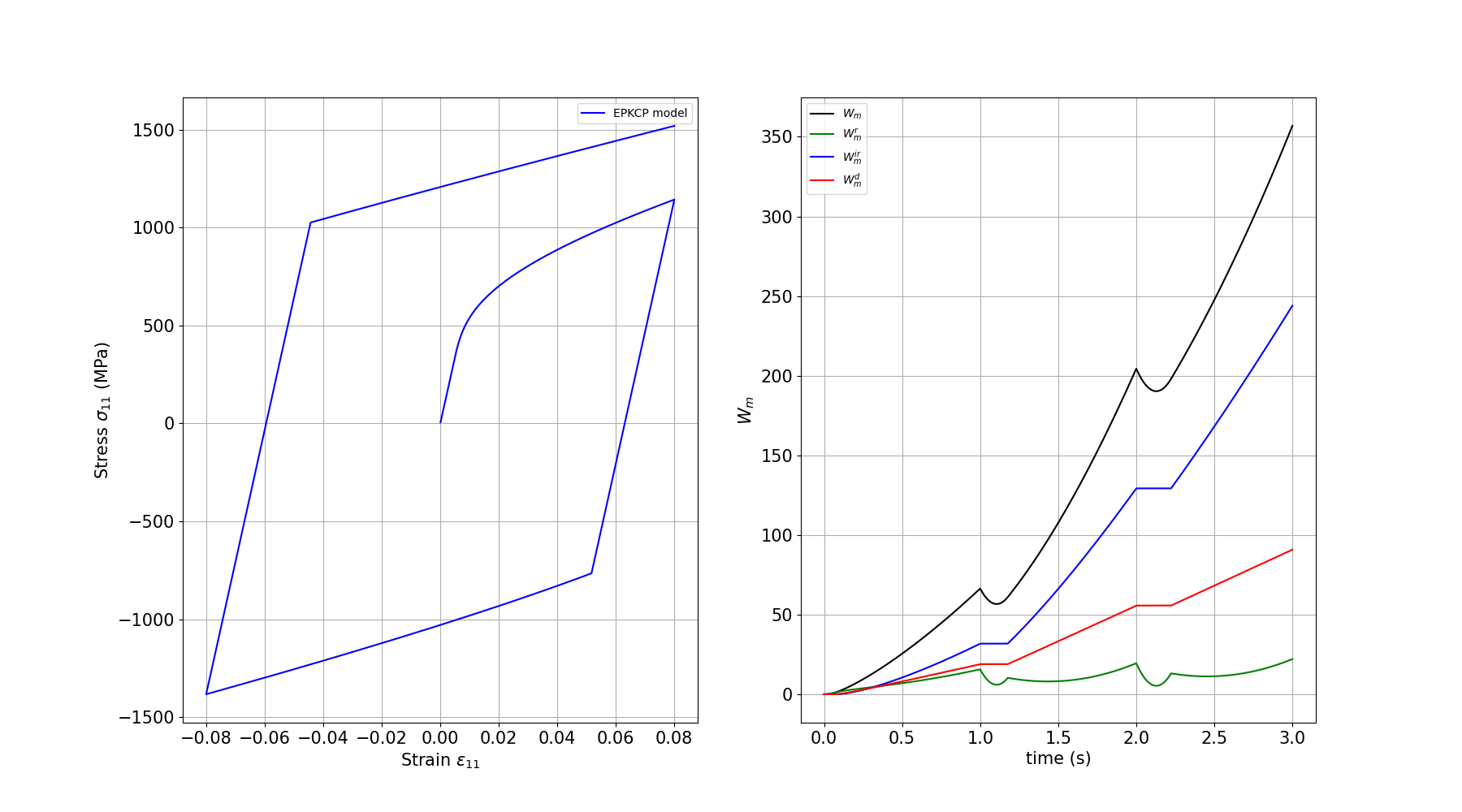
Plotting the results

We plot the stress-strain curve, the temperature evolution, the mechanical work terms and the thermal work terms.

fig = plt.figure()
outputfile_macro = os.path.join(path_results, "results_THERM_EPKCP_global-0.txt")

# Get the data
e11, e22, e33, e12, e13, e23, s11, s22, s33, s12, s13, s23 = np.loadtxt(
    outputfile_macro,
    usecols=(8, 9, 10, 11, 12, 13, 14, 15, 16, 17, 18, 19),
    unpack=True,
)
time, T, Q, r = np.loadtxt(outputfile_macro, usecols=(4, 5, 6, 7), unpack=True)
Wm, Wm_r, Wm_ir, Wm_d, Wt, Wt_r, Wt_ir = np.loadtxt(
    outputfile_macro, usecols=(20, 21, 22, 23, 24, 25, 26), unpack=True
)

# Stress vs Strain
ax = fig.add_subplot(2, 2, 1)
plt.grid(True)
plt.tick_params(axis="both", which="major", labelsize=15)
plt.xlabel(r"Strain $\varepsilon_{11}$", size=15)
plt.ylabel(r"Stress $\sigma_{11}$ (MPa)", size=15)
plt.plot(e11, s11, c="black", label="direction 1")
plt.legend(loc="best")

# Temperature vs Time
ax = fig.add_subplot(2, 2, 2)
plt.grid(True)
plt.tick_params(axis="both", which="major", labelsize=15)
plt.xlabel("time (s)", size=15)
plt.ylabel(r"Temperature $\theta$ (K)", size=15)
plt.plot(time, T, c="black", label="temperature")
plt.legend(loc="best")

# Mechanical work vs Time
ax = fig.add_subplot(2, 2, 3)
plt.grid(True)
plt.tick_params(axis="both", which="major", labelsize=15)
plt.xlabel("time (s)", size=15)
plt.ylabel(r"$W_m$", size=15)
plt.plot(time, Wm, c="black", label=r"$W_m$")
plt.plot(time, Wm_r, c="green", label=r"$W_m^r$")
plt.plot(time, Wm_ir, c="blue", label=r"$W_m^{ir}$")
plt.plot(time, Wm_d, c="red", label=r"$W_m^d$")
plt.legend(loc="best")

# Thermal work vs Time
ax = fig.add_subplot(2, 2, 4)
plt.grid(True)
plt.tick_params(axis="both", which="major", labelsize=15)
plt.xlabel("time (s)", size=15)
plt.ylabel(r"$W_t$", size=15)
plt.plot(time, Wt, c="black", label=r"$W_t$")
plt.plot(time, Wt_r, c="green", label=r"$W_t^r$")
plt.plot(time, Wt_ir, c="blue", label=r"$W_t^{ir}$")
plt.legend(loc="best")

plt.show()

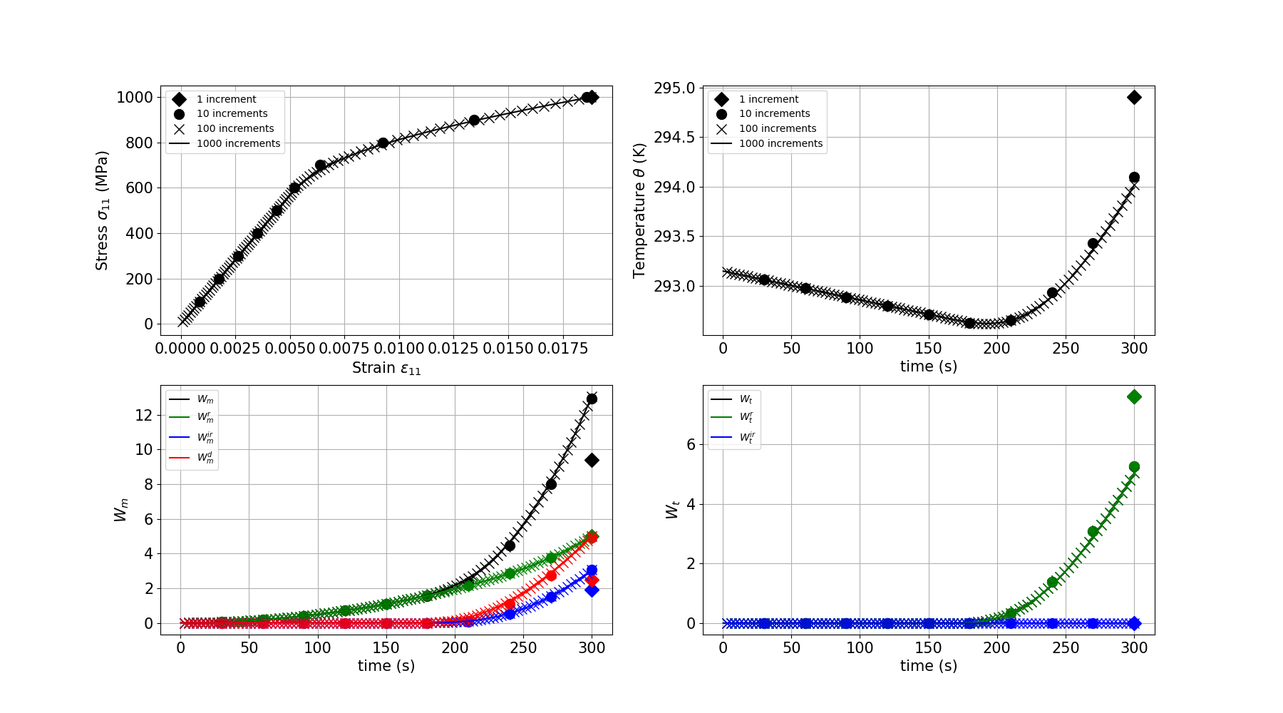
Increment size effect

Here we test the effect of the increment size on the results.

increments = [1, 10, 100, 1000]
outputfile_globals = {}

for inc in increments:
    pathfile = f"THERM_EPKCP_path_{inc}.txt"
    outputfile = f"results_THERM_EPKCP_{inc}.txt"
    sim.solver(
        umat_name,
        props,
        nstatev,
        psi_rve,
        theta_rve,
        phi_rve,
        solver_type,
        corate_type,
        path_data,
        path_results,
        pathfile,
        outputfile,
    )
    outputfile_globals[inc] = f"results_THERM_EPKCP_{inc}_global-0.txt"

# Load data for each increment
data = []
for inc in increments:
    path = os.path.join(path_results, outputfile_globals[inc])
    e11, e22, e33, e12, e13, e23, s11, s22, s33, s12, s13, s23 = np.loadtxt(
        path, usecols=range(8, 20), unpack=True
    )
    time, T, Q, r = np.loadtxt(path, usecols=range(4, 8), unpack=True)
    Wm, Wm_r, Wm_ir, Wm_d, Wt, Wt_r, Wt_ir = np.loadtxt(
        path, usecols=range(20, 27), unpack=True
    )
    data.append(
        {
            "e11": e11, "s11": s11, "time": time, "T": T,
            "Wm": Wm, "Wm_r": Wm_r, "Wm_ir": Wm_ir, "Wm_d": Wm_d,
            "Wt": Wt, "Wt_r": Wt_r, "Wt_ir": Wt_ir,
        }
    )

Plotting the increment size comparison

fig = plt.figure()

markers = ["D", "o", "x", None]
labels = ["1 increment", "10 increments", "100 increments", "1000 increments"]

# Stress vs Strain
ax = fig.add_subplot(2, 2, 1)
plt.grid(True)
plt.tick_params(axis="both", which="major", labelsize=15)
plt.xlabel(r"Strain $\varepsilon_{11}$", size=15)
plt.ylabel(r"Stress $\sigma_{11}$ (MPa)", size=15)
for i, d in enumerate(data):
    if markers[i] is not None:
        plt.plot(d["e11"], d["s11"], linestyle="None", marker=markers[i],
                 color="black", markersize=10, label=labels[i])
    else:
        plt.plot(d["e11"], d["s11"], c="black", label=labels[i])
plt.legend(loc="best")

# Temperature vs Time
ax = fig.add_subplot(2, 2, 2)
plt.grid(True)
plt.tick_params(axis="both", which="major", labelsize=15)
plt.xlabel("time (s)", size=15)
plt.ylabel(r"Temperature $\theta$ (K)", size=15)
for i, d in enumerate(data):
    if markers[i] is not None:
        plt.plot(d["time"], d["T"], linestyle="None", marker=markers[i],
                 color="black", markersize=10, label=labels[i])
    else:
        plt.plot(d["time"], d["T"], c="black", label=labels[i])
plt.legend(loc="best")

# Mechanical work vs Time
ax = fig.add_subplot(2, 2, 3)
plt.grid(True)
plt.tick_params(axis="both", which="major", labelsize=15)
plt.xlabel("time (s)", size=15)
plt.ylabel(r"$W_m$", size=15)
work_colors = ["black", "green", "blue", "red"]
work_keys = ["Wm", "Wm_r", "Wm_ir", "Wm_d"]
work_labels = [r"$W_m$", r"$W_m^r$", r"$W_m^{ir}$", r"$W_m^d$"]
for i, d in enumerate(data):
    for j, (wk, wc, wl) in enumerate(zip(work_keys, work_colors, work_labels)):
        if markers[i] is not None:
            plt.plot(d["time"], d[wk], linestyle="None", marker=markers[i],
                     color=wc, markersize=10)
        else:
            plt.plot(d["time"], d[wk], c=wc, label=wl)
plt.legend(loc="best")

# Thermal work vs Time
ax = fig.add_subplot(2, 2, 4)
plt.grid(True)
plt.tick_params(axis="both", which="major", labelsize=15)
plt.xlabel("time (s)", size=15)
plt.ylabel(r"$W_t$", size=15)
therm_keys = ["Wt", "Wt_r", "Wt_ir"]
therm_labels = [r"$W_t$", r"$W_t^r$", r"$W_t^{ir}$"]
therm_colors = ["black", "green", "blue"]
for i, d in enumerate(data):
    for j, (wk, wc, wl) in enumerate(zip(therm_keys, therm_colors, therm_labels)):
        if markers[i] is not None:
            plt.plot(d["time"], d[wk], linestyle="None", marker=markers[i],
                     color=wc, markersize=10)
        else:
            plt.plot(d["time"], d[wk], c=wc, label=wl)
plt.legend(loc="best")

plt.show()