Note
Go to the end to download the full example code.
Plasticity with isotropic hardening example
import os
import numpy as np
import matplotlib.pyplot as plt
import simcoon as sim

plt.rcParams["figure.figsize"] = (18, 10)  # configure the figure output size

plt.rc("text", usetex=True)
plt.rc("font", family="serif")

# ###################################################################################
# The elastic-plastic (isotropic hardening) constitutive law implemented in Simcoon is a rate independent, isotropic, von Mises type material with power-law isotropic hardening.
# Eight parameters are required for the thermomechanical version:
# The parameters required are:
#
# 1. The density :math:`\rho`
# 2. The specific heat :math:`c_p`
# 3. The Young modulus :math:`E`
# 4. The Poisson ratio :math:`\nu`
# 5. The coefficient of thermal expansion :math:`\alpha`
# 6. The von Mises equivalent yield stress limit :math:`\sigma_{Y}`
# 7. The hardening parameter :math:`k`
# 8. The hardening exponent :math:`m`
#
# The constitutive law is given by the set of equations :
#
# .. math::
#
#   {\sigma}_{ij} & = L_{ijkl}\left({\varepsilon}^{\textrm{tot}}_{kl}-\alpha_{kl}\left(T-T^{\textrm{ref}}\right)-{\varepsilon}^{\textrm{p}}_{kl}\right) \\\\
#   \dot{\varepsilon}^{\textrm{p}}_{ij} & =\dot{p}\Lambda_{ij}, \quad \Lambda_{ij}=\frac{3}{2}\frac{\sigma'_{ij}}{\overline{\sigma}}, \quad \sigma'_{ij}=\sigma_{ij}-\frac{1}{3}\sigma_{kk}\delta_{ij}, \quad \overline{\sigma}=\sqrt{\frac{3}{2}\sigma'_{kl}\sigma'_{kl}}, \\\\
#   \Phi & =\overline{\sigma}-\sigma_{Y}-kp^m\leq 0, \quad \dot{p}\geq0,~~~ \dot{p}~\Phi=0
#
# where :math:`{\varepsilon}^{\textrm{p}}_{ij}` is the plastic strain tensor, :math:`p` is the plastic multiplier,
# :math:`\sigma'_{ij}` is the deviatoric part of the stress and :math:`\overline{\sigma}` is the von Mises equivalent
# stress (Lemaitre and Chaboche, 2002). Moreover, :math:`T^{\textrm{ref}}` is a reference temperature
# (usually the temperature at the beginning of the analysis).
#
# In Simcoon the elastoplastic material constitutive law is implemented using a *return mapping algorithm*,
# with use of the *convex cutting plane* algorithm (Simo and Hughes, 1998). The updated stress is provided for 1D,
# plane stress, and generalized plane strain/3D analysis according to the forms of elastic isotropic materials.
#
# The updated work, and internal heat production :math:`r` are determined with the algorithm presented in the *simcoon* documentation.
#
# As a start we should input the name of the UMAT as well as the list of parameters

umat_name = "EPICP"  # This is the 5 character code for the elastic-plastic subroutine
nstatev = 8  # The number of scalar variables required, only the initial temperature is stored here

E = 113800
nu = 0.342
alpha = 0.86e-5
sigma_Y = 600
H = 1600
beta = 0.25

psi_rve = 0.0
theta_rve = 0.0
phi_rve = 0.0
solver_type = 0
corate_type = 3

# Define the properties
props = np.array([E, nu, alpha, sigma_Y, H, beta])
path_data = "../data"

# Run the simulation: the loading path is read in Python and the case runs in
# memory, so no result file is written.
pathfile = "EPICP_path.json"
blocks, T_init, _ = sim.solver.load_path_json(os.path.join(path_data, pathfile))
res = sim.solver.solve(
    blocks,
    umat_name,
    props,
    nstatev,
    T_init=T_init,
    solver_type=solver_type,
    corate=corate_type,
    orientation=(psi_rve, theta_rve, phi_rve),
)

# ###################################################################################
# Plotting the results
# --------------------------------------
# This is it, now we just need to plot the results.
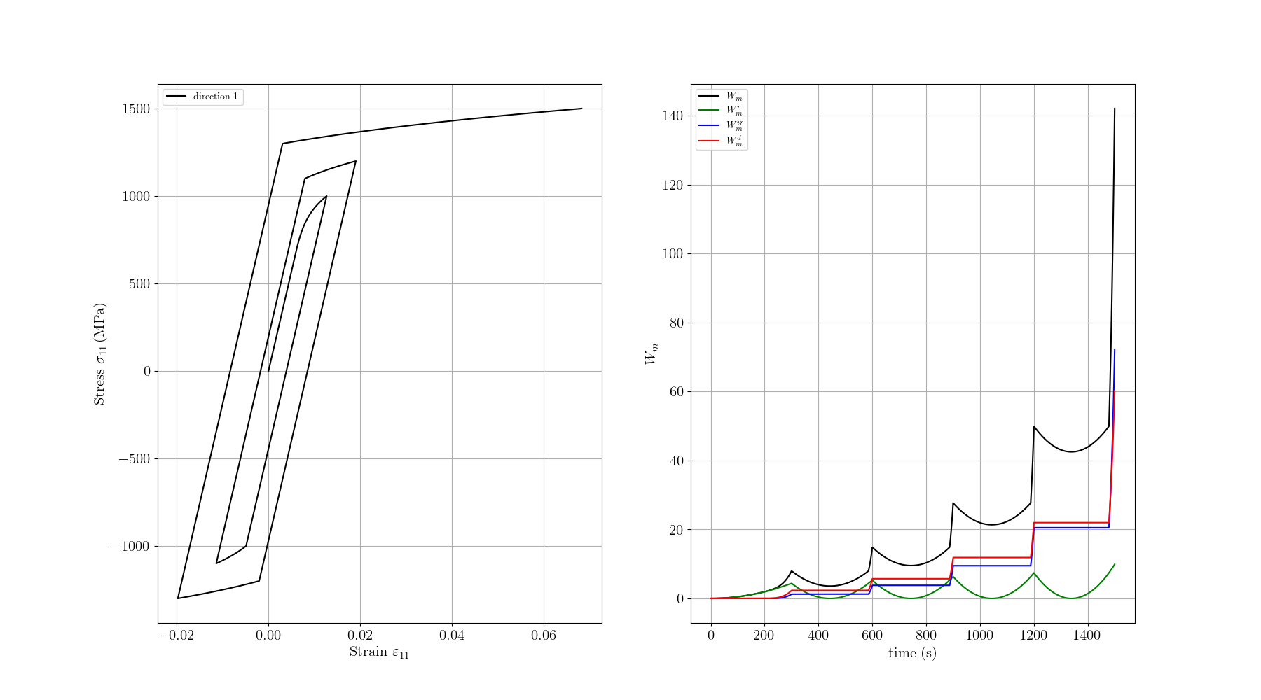
# In the left, we plot the stress vs strain curve, and in the right the different work terms vs time:
# - :meth:`Wm <simcoon.Wm>` the mechanical work,
# - :meth:`Wm_r <simcoon.Wm_r>` the recoverable mechanical work,
# - :meth:`Wm_ir <simcoon.Wm_ir>` the irrecoverable mechanical work,
# - :meth:`Wm_d <simcoon.Wm_d>` the dissipated mechanical work.
# ###################################################################################

# prepare the load
fig = plt.figure()

# Get the data
e11, e22, e33, e12, e13, e23 = res["Strain"]
s11, s22, s33, s12, s13, s23 = res["Stress"]
time, T = res["Time"], res["Temp"]
Wm, Wm_r, Wm_ir, Wm_d = res["Wm"]

# Plot the results
ax = fig.add_subplot(1, 2, 1)
plt.grid(True)
plt.tick_params(axis="both", which="major", labelsize=15)
plt.xlabel(r"Strain $\varepsilon_{11}$", size=15)
plt.ylabel(r"Stress $\sigma_{11}$\,(MPa)", size=15)
plt.plot(e11, s11, c="black", label="direction 1")
plt.legend(loc=2)

ax = fig.add_subplot(1, 2, 2)
plt.grid(True)
plt.tick_params(axis="both", which="major", labelsize=15)
plt.xlabel("time (s)", size=15)
plt.ylabel(r"$W_m$", size=15)
plt.plot(time, Wm, c="black", label=r"$W_m$")
plt.plot(time, Wm_r, c="green", label=r"$W_m^r$")
plt.plot(time, Wm_ir, c="blue", label=r"$W_m^{ir}$")
plt.plot(time, Wm_d, c="red", label=r"$W_m^d$")
plt.legend(loc=2)

plt.show()

# ###################################################################################
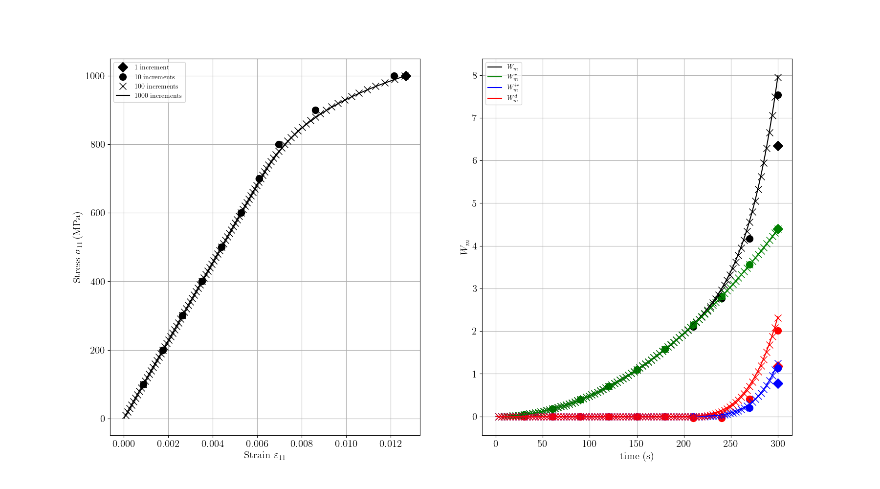
# Here we test the increment size effect on the results
# ----------------------------------------------------------
# ###################################################################################

# Define the increment counts to compare
increments = [1, 10, 100, 1000]

# Run each case and collect its history: every path file is parsed in Python and
# the case runs in memory, so nothing is written to — or read back from — disk.
data = []
for inc in increments:
    pathfile = f"EPICP_path_{inc}.json"
    blocks, T_init, _ = sim.solver.load_path_json(os.path.join(path_data, pathfile))
    res_inc = sim.solver.solve(
        blocks,
        umat_name,
        props,
        nstatev,
        T_init=T_init,
        solver_type=solver_type,
        corate=corate_type,
        orientation=(psi_rve, theta_rve, phi_rve),
    )
    Wm_i, Wm_r_i, Wm_ir_i, Wm_d_i = res_inc["Wm"]
    data.append(
        {
            "e11": res_inc["Strain"][0],
            "s11": res_inc["Stress"][0],
            "time": res_inc["Time"],
            "Wm": Wm_i,
            "Wm_r": Wm_r_i,
            "Wm_ir": Wm_ir_i,
            "Wm_d": Wm_d_i,
        }
    )

# ###################################################################################
# Plotting the results
# --------------------------------------
#
# In the left, we plot the stress vs strain curve, and in the right the different work terms vs time
# Note the ["D", "o", "x", None] markers used to differentiate the different increment sizes:
# ["1 increment", "10 increments", "100 increments", "1000 increments"]
#
# ###################################################################################

fig = plt.figure()

markers = ["D", "o", "x", None]
labels = ["1 increment", "10 increments", "100 increments", "1000 increments"]
colors = ["black", "black", "black", "black"]

# First subplot: Stress vs Strain
ax1 = fig.add_subplot(1, 2, 1)
plt.grid(True)
plt.tick_params(axis="both", which="major", labelsize=15)
plt.xlabel(r"Strain $\varepsilon_{11}$", size=15)
plt.ylabel(r"Stress $\sigma_{11}$\,(MPa)", size=15)

for i, d in enumerate(data):
    if markers[i] is not None:
        plt.plot(
            d["e11"],
            d["s11"],
            linestyle="None",
            marker=markers[i],
            color=colors[i],
            markersize=10,
            label=labels[i],
        )
    else:
        plt.plot(d["e11"], d["s11"], c=colors[i], label=labels[i])
plt.legend(loc=2)

# Second subplot: Work terms vs Time
ax2 = fig.add_subplot(1, 2, 2)
plt.grid(True)
plt.tick_params(axis="both", which="major", labelsize=15)
plt.xlabel("time (s)", size=15)
plt.ylabel(r"$W_m$", size=15)

work_colors = ["black", "green", "blue", "red"]
work_keys = ["Wm", "Wm_r", "Wm_ir", "Wm_d"]
work_labels = [r"$W_m$", r"$W_m^r$", r"$W_m^{ir}$", r"$W_m^d$"]

for i, d in enumerate(data):
    for j, (wk, wc, wl) in enumerate(zip(work_keys, work_colors, work_labels)):
        if markers[i] is not None:
            plt.plot(
                d["time"],
                d[wk],
                linestyle="None",
                marker=markers[i],
                color=wc,
                markersize=10,
                label=wl if i == len(data) - 1 else None,  # Only label once
            )
        else:
            plt.plot(d["time"], d[wk], c=wc, label=wl)
plt.legend(loc=2)

plt.show()
#
Total running time of the script: (0 minutes 2.970 seconds)