J2 plasticity written in Python (PYEXT)

A constitutive law implemented in numpy and integrated by the C++ solver through the PYEXT callback: radial-return J2 plasticity with linear isotropic hardening and the consistent (Simo-Hughes) tangent, compared with the built-in EPICP kernel (power-law hardening with exponent m = 1).

import matplotlib.pyplot as plt
import numpy as np

import simcoon as sim
from simcoon.solver import Block, StepMeca, solve

The law

A simcoon.PythonUMAT receives the state at the beginning of the increment (Etot, sigma, statev, Wm), the increment DEtot and returns (sigma, Lt, statev, Wm[, L]). Everything the law must remember lives in statev (here the cumulated plastic strain p and the plastic strain tensor): the solver re-calls the same increment during its Newton iterations with statev reset to its start-of-increment value.

E, NU, SIGMA_Y, K_HARD = 70000.0, 0.3, 300.0, 1000.0
ENG_SHEAR = np.array([1.0, 1.0, 1.0, 2.0, 2.0, 2.0])   # stress-like -> strain-like Voigt vector


class J2Linear(sim.PythonUMAT):
    nstatev = 7            # p, EP(6)

    def __init__(self, E, nu, sigma_y, k):
        self.L = sim.L_iso([E, nu], "Enu")
        self.G = E / (2.0 * (1.0 + nu))
        self.K = E / (3.0 * (1.0 - 2.0 * nu))
        self.sigma_y, self.k = sigma_y, k
        # projectors of the tangent (they act on strain-like vectors)
        self.Idev = sim.Tensor4.deviatoric("stiffness").mat
        self.Ivol = sim.Tensor4.volumetric("stiffness").mat

    def integrate(self, *, Etot, DEtot, sigma, statev, Wm, tangent_mode, **kw):
        p, EP = statev[0], statev[1:7]
        eps = Etot + DEtot
        L, G, k = self.L, self.G, self.k
        sig_tr = L @ (eps - EP)
        s_tr = sig_tr.copy()
        s_tr[:3] -= sig_tr[:3].mean()          # stress deviator (not a stiffness projector: it
                                               # would halve the shear stresses)
        norm_s = np.sqrt(s_tr[:3] @ s_tr[:3] + 2.0 * (s_tr[3:] @ s_tr[3:]))
        q_tr = np.sqrt(1.5) * norm_s
        f = q_tr - (self.sigma_y + k * p)
        stress, Lt = sig_tr, L
        if f > 0.0:
            dp = f / (3.0 * G + k)
            n = s_tr / norm_s
            stress = sig_tr - 2.0 * G * dp * np.sqrt(1.5) * n
            EP = EP + dp * np.sqrt(1.5) * n * ENG_SHEAR
            p = p + dp
            if tangent_mode != 0:
                beta = 1.0 - 3.0 * G * dp / q_tr
                gamma = 3.0 * G / (3.0 * G + k) - (1.0 - beta)
                Lt = (3.0 * self.K * self.Ivol + 2.0 * G * beta * self.Idev
                      - 2.0 * G * gamma * np.outer(n, n * ENG_SHEAR))
        Wm = Wm.copy()
        Wm[0] += 0.5 * (sigma + stress) @ DEtot
        return stress, Lt, np.concatenate([[p], EP]), Wm, L

Cyclic uniaxial loading under mixed control

The axial strain is prescribed, the five other stress components are driven to zero: the tangent returned by the law feeds the Newton loop of the solver.

uniaxial = ["strain"] + ["stress"] * 5
load = StepMeca(control=uniaxial, value=[0.02, 0, 0, 0, 0, 0], ninc=40)
reverse = StepMeca(control=uniaxial, value=[-0.02, 0, 0, 0, 0, 0], ninc=40)
blocks = [Block(steps=[load, reverse], ncycle=2)]

res_py = solve(blocks, J2Linear(E, NU, SIGMA_Y, K_HARD))
res_ref = solve(blocks, "EPICP", [E, NU, 1.0e-5, SIGMA_Y, K_HARD, 1.0], 8)

print("max |sigma_py - sigma_EPICP| =", np.abs(res_py["Stress"] - res_ref["Stress"]).max(), "MPa")
print("max |p_py - p_EPICP|         =", np.abs(res_py["Statev"][0] - res_ref["Statev"][1]).max())

fig, ax = plt.subplots(figsize=(6, 4))
ax.plot(res_ref["Strain"][0], res_ref["Stress"][0], "k-", lw=2, label="EPICP (C++)")
ax.plot(res_py["Strain"][0], res_py["Stress"][0], "r--", lw=1.5, label="J2 in numpy (PYEXT)")
ax.set_xlabel(r"$\varepsilon_{11}$")
ax.set_ylabel(r"$\sigma_{11}$ (MPa)")
ax.grid(True)
ax.legend()
fig.tight_layout()
plt.show()

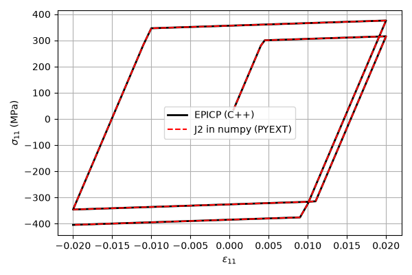
max |sigma_py - sigma_EPICP| = 4.1592329580453224e-10 MPa
max |p_py - p_EPICP|         = 4.62088700636798e-13