A Neo-Hookean material with the Tensor API

One constitutive law, every measure: this example defines a compressible Neo-Hookean hyperelastic law and uses the typed Tensor2 / Tensor4 classes to move stresses, strains and tangents between the reference and the current configuration.

The strain energy is the classical compressible Neo-Hookean potential

\[W = \frac{\mu}{2}\,(I_1 - 3) - \mu \ln J + \frac{\lambda}{2}\,(\ln J)^2,\]

which gives closed forms in both configurations:

\[\mathbf{S} = \mu\,(\mathbf{I} - \mathbf{C}^{-1}) + \lambda \ln J\, \mathbf{C}^{-1} \qquad\text{(PKII, reference)}\]

\[\boldsymbol{\tau} = \mu\,(\mathbf{b} - \mathbf{I}) + \lambda \ln J\, \mathbf{I} \qquad\text{(Kirchhoff, current)}\]

so every push-forward / pull-back performed with the Tensor API can be checked against an exact analytical result.

Voigt order is the simcoon convention [11, 22, 33, 12, 13, 23].

import numpy as np
import simcoon as sim

0. Material and deformation

A rubber-like compressible Neo-Hookean solid (units: MPa), and a deformation gradient combining stretch and shear so that nothing is orthogonal and J = det(F) != 1 (all the metric factors matter).

E_mod = 10.0     # Young modulus (MPa)
nu = 0.45        # Poisson ratio
mu = E_mod / (2.0 * (1.0 + nu))            # shear modulus
lam = E_mod * nu / ((1.0 + nu) * (1.0 - 2.0 * nu))  # Lame first parameter

F = np.array([[1.30, 0.20, 0.00],
              [0.00, 0.95, 0.10],
              [0.00, 0.00, 0.90]])
J = np.linalg.det(F)
I3 = np.eye(3)

C = F.T @ F                     # right Cauchy-Green
b = F @ F.T                     # left Cauchy-Green
Cinv = np.linalg.inv(C)

print(f"mu = {mu:.4f} MPa, lambda = {lam:.4f} MPa, J = {J:.4f}")

mu = 3.4483 MPa, lambda = 31.0345 MPa, J = 1.1115

1. Strain measures and their transport

Green-Lagrange E lives in the reference configuration, Euler-Almansi e in the current one. They are the same covariant object seen from the two configurations: the strain push-forward F^{-T} E F^{-1} maps one exactly onto the other (no J factor is involved for strains).

E_GL = sim.Tensor2.strain(sim.Green_Lagrange(F))
e_EA = sim.Tensor2.strain(sim.Euler_Almansi(F))

e_from_E = E_GL.push_forward(F)
E_from_e = e_EA.pull_back(F)

print("push_forward(E) == e (Euler-Almansi):",
      np.allclose(e_from_E.mat, e_EA.mat))
print("pull_back(e)    == E (Green-Lagrange):",
      np.allclose(E_from_e.mat, E_GL.mat))

# The logarithmic (Hencky) strain ln V is a third measure, living in the
# current configuration -- it is the one simcoon's solver works with.
h = sim.Tensor2.strain(sim.Log_strain(F))
print("Hencky strain ln V (Voigt):", np.round(h.voigt, 4))

push_forward(E) == e (Euler-Almansi): True
pull_back(e)    == E (Green-Lagrange): True
Hencky strain ln V (Voigt): [ 0.2695 -0.0555 -0.1083  0.1503 -0.0072  0.106 ]

2. The law in the reference configuration: PKII stress

S = mu (I - C^{-1}) + lambda ln(J) C^{-1}

S_mat = mu * (I3 - Cinv) + lam * np.log(J) * Cinv
S = sim.Tensor2.stress(S_mat)
print("S (PKII, Voigt):", np.round(S.voigt, 4))

S (PKII, Voigt): [ 3.3447  3.2603  3.2414  0.0289 -0.0034  0.0218]

3. The same law in the current configuration: Kirchhoff stress

tau = mu (b - I) + lambda ln(J) I – this is F S F^T, computed directly.

tau_mat = mu * (b - I3) + lam * np.log(J) * I3
tau = sim.Tensor2.stress(tau_mat)

4. Stress transport: one object, three measures

For a stress the push-forward is the Piola transformation F () F^T, and the metric flag decides the J factor:

• metric=False : S -> tau (Kirchhoff, per reference volume)

• metric=True : S -> sigma (Cauchy, per current volume)

tau_from_S = S.push_forward(F, metric=False)
sigma_from_S = S.push_forward(F, metric=True)

print("push_forward(S, metric=False) == tau  :",
      np.allclose(tau_from_S.mat, tau.mat))
print("push_forward(S, metric=True)  == tau/J:",
      np.allclose(sigma_from_S.mat, tau.mat / J))
print("pull_back(tau) == S (round trip)      :",
      np.allclose(tau.pull_back(F, metric=False).mat, S.mat))

sigma = sigma_from_S
print("\nCauchy sigma (Voigt):", np.round(sigma.voigt, 4))
print("von Mises (Cauchy):", np.round(sigma.mises(), 4), "MPa")

push_forward(S, metric=False) == tau  : True
push_forward(S, metric=True)  == tau/J: True
pull_back(tau) == S (round trip)      : True

Cauchy sigma (Voigt): [ 5.2163  2.6801  2.3621  0.5894 -0.      0.2792]
von Mises (Cauchy): 2.9353 MPa

5. The material tangent dS/dE

The Neo-Hookean referential tangent is also closed-form:

dS/dE = lambda C^{-1} (x) C^{-1} + 2 (mu - lambda ln J) C^{-1} (.) C^{-1}

where (x) is the dyadic product and (.) the symmetrized dyadic operator (a (.) a)_{ijkl} = 1/2 (a_ik a_jl + a_il a_jk), available as sim.auto_sym_dyadic_operator.

cinv_v = sim.t2v_stress(Cinv).ravel()   # raw-component Voigt of C^{-1}
dSdE_mat = (lam * np.outer(cinv_v, cinv_v)
            + 2.0 * (mu - lam * np.log(J)) * sim.auto_sym_dyadic_operator(Cinv))
dSdE = sim.Tensor4.stiffness(dSdE_mat)

# Numerical verification by central differences on S(E), perturbing the
# engineering Voigt strain components.
def S_of_E(E_voigt_eng):
    C_pert = 2.0 * sim.v2t_strain(E_voigt_eng) + I3
    Cinv_pert = np.linalg.inv(C_pert)
    J_pert = np.sqrt(np.linalg.det(C_pert))
    return sim.t2v_stress(mu * (I3 - Cinv_pert)
                          + lam * np.log(J_pert) * Cinv_pert).ravel()

E_v = E_GL.voigt
h_step = 1e-6
dSdE_num = np.empty((6, 6))
for j in range(6):
    dE = np.zeros(6)
    dE[j] = h_step
    dSdE_num[:, j] = (S_of_E(E_v + dE) - S_of_E(E_v - dE)) / (2.0 * h_step)

print("analytic dS/dE == numerical dS/dE:",
      np.allclose(dSdE.mat, dSdE_num, rtol=1e-5, atol=1e-6))

# Sanity check: at F = I the tangent must reduce to the isotropic linear
# elastic stiffness with the same Lame constants.
dSdE_at_I = (lam * np.outer(sim.t2v_stress(I3), sim.t2v_stress(I3))
             + 2.0 * mu * sim.auto_sym_dyadic_operator(I3))
print("dS/dE at F=I == L_iso(E, nu):",
      np.allclose(dSdE_at_I, sim.L_iso([E_mod, nu], "Enu")))

analytic dS/dE == numerical dS/dE: True
dS/dE at F=I == L_iso(E, nu): True

6. Tangent transport: from dS/dE to the spatial moduli

A stiffness push-forward drags all four legs by F. For the Neo-Hookean tangent the result is again closed-form, because the push-forward of C^{-1} is the identity (F C^{-1} F^T = I):

c_tau = lambda I (x) I + 2 (mu - lambda ln J) I_sym (metric=False)

i.e. the spatial (Lie-rate / Oldroyd) Kirchhoff tangent looks like an isotropic stiffness with effective Lame constants (lambda, mu - lambda lnJ). With metric=True everything is divided by J (Cauchy scaling).

c_tau = dSdE.push_forward(F, metric=False)

c_tau_expected = (lam * np.outer(sim.t2v_stress(I3), sim.t2v_stress(I3))
                  + 2.0 * (mu - lam * np.log(J)) * sim.auto_sym_dyadic_operator(I3))
print("push_forward(dS/dE, metric=False) == lambda IxI + 2(mu - lambda lnJ) Isym:",
      np.allclose(c_tau.mat, c_tau_expected))

c_sigma = dSdE.push_forward(F, metric=True)
print("metric=True is the same tangent / J:",
      np.allclose(c_sigma.mat, c_tau.mat / J))

# The round trip back to the reference configuration is exact as well.
print("pull_back(c_tau) == dS/dE (round trip):",
      np.allclose(c_tau.pull_back(F, metric=False).mat, dSdE.mat))

# Note: this spatial tangent is conjugate to the Lie (Truesdell/Oldroyd) rate.
# The tangents conjugate to the Jaumann, Green-Naghdi or logarithmic rates add
# a stress-dependent correction (CoRate overload of tensor4::push_forward on
# the C++ side, matching the solver's per-corate dispatch).

push_forward(dS/dE, metric=False) == lambda IxI + 2(mu - lambda lnJ) Isym: True
metric=True is the same tangent / J: True
pull_back(c_tau) == dS/dE (round trip): True

7. Batch: a full uniaxial-stretch curve in three stress measures

The same Tensor calls accept batches. Sweep a confined uniaxial stretch F = diag(lambda_1, 1, 1) (so J = lambda_1 != 1 and the measures separate), build the (N,6) PKII batch with plain numpy, then transport the whole batch with one call.

N = 80
lam1 = np.linspace(0.70, 1.60, N)
F_batch = np.zeros((N, 3, 3))
F_batch[:, 0, 0] = lam1
F_batch[:, 1, 1] = 1.0
F_batch[:, 2, 2] = 1.0
J_batch = lam1

C11 = lam1**2
S11 = mu * (1.0 - 1.0 / C11) + lam * np.log(J_batch) / C11
S22 = lam * np.log(J_batch)                     # C22 = 1 -> mu term vanishes
S_voigt = np.zeros((N, 6))
S_voigt[:, 0] = S11
S_voigt[:, 1] = S22
S_voigt[:, 2] = S22

S_b = sim.Tensor2.stress(S_voigt)              # batch of N PKII tensors
tau_b = S_b.push_forward(F_batch, metric=False)   # batch Kirchhoff
sigma_b = S_b.push_forward(F_batch, metric=True)  # batch Cauchy

print("batch:", len(S_b), "points, von Mises range:",
      np.round(sigma_b.mises().min(), 3), "->",
      np.round(sigma_b.mises().max(), 3), "MPa")

import matplotlib.pyplot as plt

fig, ax = plt.subplots(figsize=(7.0, 4.5))
ax.plot(lam1, S_b.voigt[:, 0], "-.^", ms=3, label="PKII $S_{11}$ (reference)")
ax.plot(lam1, tau_b.voigt[:, 0], ":d", ms=3, label=r"Kirchhoff $\tau_{11}$")
ax.plot(lam1, sigma_b.voigt[:, 0], "-o", ms=3, label=r"Cauchy $\sigma_{11}$")
ax.axhline(0.0, color="k", lw=0.5)
ax.axvline(1.0, color="k", lw=0.5)
ax.set_xlabel(r"Stretch $\lambda_1$  (confined uniaxial, $J = \lambda_1$)")
ax.set_ylabel("Stress (MPa)")
ax.set_title("Neo-Hookean: one law, three stress measures")
ax.grid(True, alpha=0.3)
ax.legend(fontsize=9)
fig.tight_layout()
plt.show()

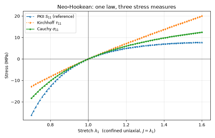
batch: 80 points, von Mises range: 0.026 -> 3.362 MPa