Shape Memory Alloy - Superelastic Model

import numpy as np
import matplotlib.pyplot as plt
import simcoon as sim
import os

plt.rcParams["figure.figsize"] = (18, 10)

The SMA (Shape Memory Alloy) transformation constitutive law is a rate-independent description of the austenite-martensite phase transformation. Both forward (austenite to martensite) and reverse (martensite to austenite) transformations are treated as independent mechanisms.

Twenty-eight parameters are required:

1. \(\mathrm{flagT}\) : Temperature extrapolation flag (0: linear, 1: smooth)

2. \(E_A\) : Young’s modulus of austenite

3. \(E_M\) : Young’s modulus of martensite

4. \(\nu_A\) : Poisson’s ratio of austenite

5. \(\nu_M\) : Poisson’s ratio of martensite

6. \(\alpha_A\) : CTE of austenite

7. \(\alpha_M\) : CTE of martensite

8. \(H_{\min}\) : Minimal transformation strain magnitude

9. \(H_{\max}\) : Maximal transformation strain magnitude

10. \(k_1\) : Exponential evolution of transformation strain

11. \(\sigma_{\mathrm{crit}}\) : Critical stress for transformation strain change

12. \(C_A\) : Clausius-Clapeyron slope (martensite to austenite)

13. \(C_M\) : Clausius-Clapeyron slope (austenite to martensite)

14. \(M_{s0}\) : Martensite start temperature at zero stress

15. \(M_{f0}\) : Martensite finish temperature at zero stress

16. \(A_{s0}\) : Austenite start temperature at zero stress

17. \(A_{f0}\) : Austenite finish temperature at zero stress

18. \(n_1\) : Martensite start smooth exponent

19. \(n_2\) : Martensite finish smooth exponent

20. \(n_3\) : Austenite start smooth exponent

21. \(n_4\) : Austenite finish smooth exponent

22. \(\sigma_{\mathrm{caliber}}\) : Calibration stress

23. \(b_{\mathrm{Prager}}\) : Prager parameter

24. \(n_{\mathrm{Prager}}\) : Prager exponent

25. \(c_{\lambda}\) : Penalty function exponent start point

26. \(p_{0,\lambda}\) : Penalty function limit value

27. \(n_{\lambda}\) : Penalty function power law exponent

28. \(\alpha_{\lambda}\) : Penalty function power law parameter

The constitutive law uses a return mapping algorithm with a convex cutting plane method (Simo and Hughes, 1998). The superelastic response exhibits a stress-induced phase transformation loop.

umat_name = "SMAUT"  # 5 character code for the SMA transformation model
nstatev = 50  # Number of internal state variables

# Material parameters
flagT = 0  # Temperature extrapolation flag
E_A = 67538.0  # Young's modulus of austenite (MPa)
E_M = 67538.0  # Young's modulus of martensite (MPa)
nu_A = 0.349  # Poisson's ratio of austenite
nu_M = 0.349  # Poisson's ratio of martensite
alphaA = 1.0e-6  # CTE of austenite
alphaM = 1.0e-6  # CTE of martensite
Hmin = 0.0  # Minimal transformation strain
Hmax = 0.0418  # Maximal transformation strain
k1 = 0.021  # Exponential evolution parameter
sigmacrit = 0.0  # Critical stress
C_A = 10.0  # Clausius-Clapeyron slope (M -> A)
C_M = 10.0  # Clausius-Clapeyron slope (A -> M)
Ms0 = 250.0  # Martensite start temperature (K)
Mf0 = 230.0  # Martensite finish temperature (K)
As0 = 260.0  # Austenite start temperature (K)
Af0 = 280.0  # Austenite finish temperature (K)
n1 = 0.2  # Martensite start smooth exponent
n2 = 0.2  # Martensite finish smooth exponent
n3 = 0.2  # Austenite start smooth exponent
n4 = 0.2  # Austenite finish smooth exponent
sigmacaliber = 300.0  # Calibration stress (MPa)
b_prager = 1.4  # Prager parameter
n_prager = 2.0  # Prager exponent
c_lambda = 1.0e-6  # Penalty function start point
p0_lambda = 1.0e-3  # Penalty function limit value
n_lambda = 1.0  # Penalty function power law exponent
alpha_lambda = 1.0e8  # Penalty function power law parameter

psi_rve = 0.0
theta_rve = 0.0
phi_rve = 0.0
solver_type = 0
corate_type = 3

props = np.array([
    flagT, E_A, E_M, nu_A, nu_M, alphaA, alphaM,
    Hmin, Hmax, k1, sigmacrit,
    C_A, C_M, Ms0, Mf0, As0, Af0,
    n1, n2, n3, n4,
    sigmacaliber, b_prager, n_prager,
    c_lambda, p0_lambda, n_lambda, alpha_lambda,
])

path_data = "../data"
path_results = "results"
pathfile = "SMAUT_path.txt"
outputfile = "results_SMAUT.txt"

sim.solver(
    umat_name,
    props,
    nstatev,
    psi_rve,
    theta_rve,
    phi_rve,
    solver_type,
    corate_type,
    path_data,
    path_results,
    pathfile,
    outputfile,
)

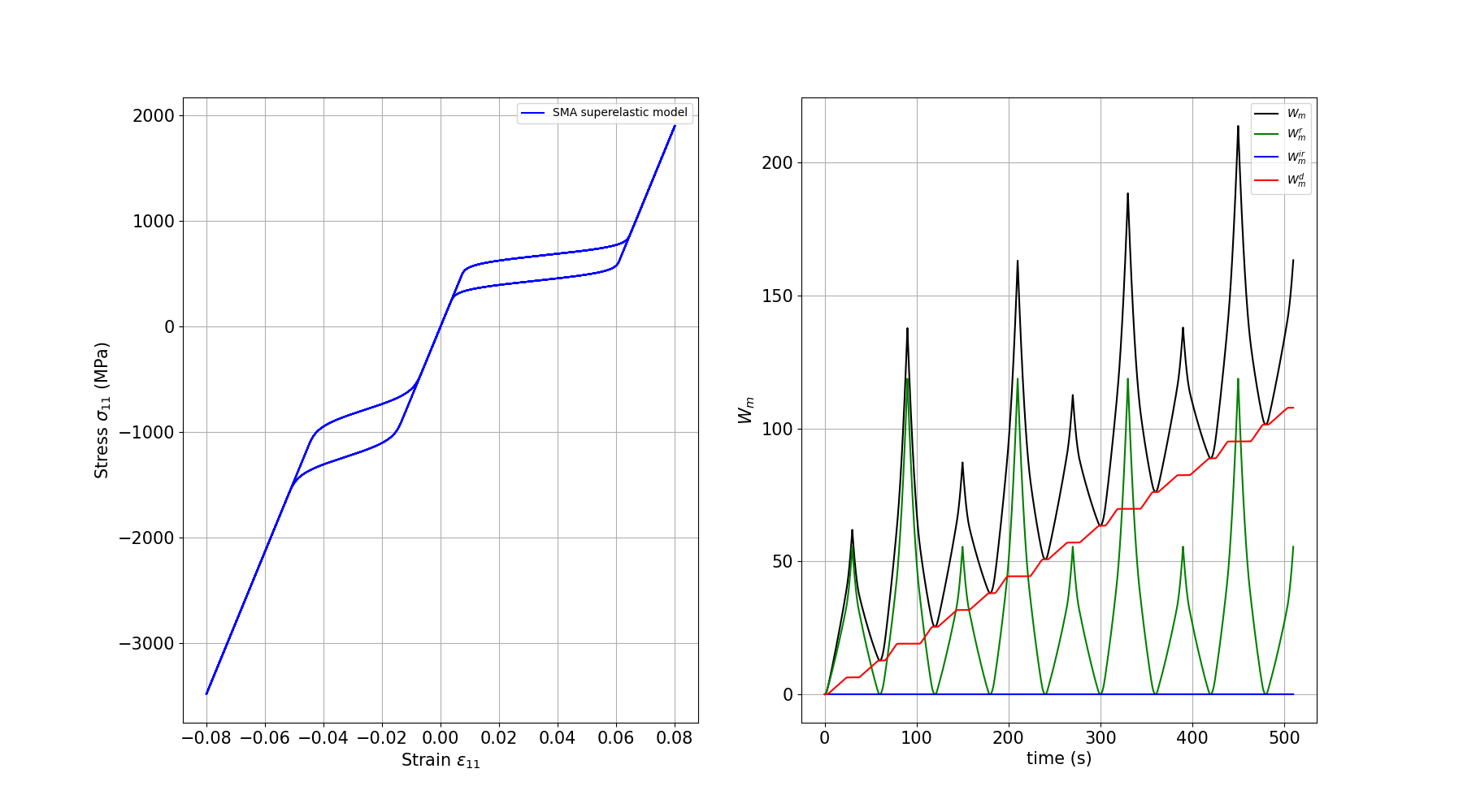
Plotting the results

We plot the superelastic stress-strain loop which shows the stress-induced austenite-martensite phase transformation and its reverse upon unloading.

outputfile_macro = os.path.join(path_results, "results_SMAUT_global-0.txt")

fig = plt.figure()

e11, e22, e33, e12, e13, e23, s11, s22, s33, s12, s13, s23 = np.loadtxt(
    outputfile_macro,
    usecols=(8, 9, 10, 11, 12, 13, 14, 15, 16, 17, 18, 19),
    unpack=True,
)
time, T, Q_out, r = np.loadtxt(outputfile_macro, usecols=(4, 5, 6, 7), unpack=True)
Wm, Wm_r, Wm_ir, Wm_d = np.loadtxt(
    outputfile_macro, usecols=(20, 21, 22, 23), unpack=True
)

# First subplot: Stress vs Strain (superelastic loop)
ax1 = fig.add_subplot(1, 2, 1)
plt.grid(True)
plt.tick_params(axis="both", which="major", labelsize=15)
plt.xlabel(r"Strain $\varepsilon_{11}$", size=15)
plt.ylabel(r"Stress $\sigma_{11}$ (MPa)", size=15)
plt.plot(e11, s11, c="blue", label="SMA superelastic model")
plt.legend(loc="best")

# Second subplot: Work terms vs Time
ax2 = fig.add_subplot(1, 2, 2)
plt.grid(True)
plt.tick_params(axis="both", which="major", labelsize=15)
plt.xlabel("time (s)", size=15)
plt.ylabel(r"$W_m$", size=15)
plt.plot(time, Wm, c="black", label=r"$W_m$")
plt.plot(time, Wm_r, c="green", label=r"$W_m^r$")
plt.plot(time, Wm_ir, c="blue", label=r"$W_m^{ir}$")
plt.plot(time, Wm_d, c="red", label=r"$W_m^d$")
plt.legend(loc="best")

plt.show()