Note
Go to the end to download the full example code.
Shape Memory Alloy - Thermomechanical coupling
import numpy as np
import matplotlib.pyplot as plt
import simcoon as sim
import os

plt.rcParams["figure.figsize"] = (18, 10)
The SMA (transformation-only) constitutive law implemented in simcoon is a rate independent description of phase transformation where two transformations (austenite to martensite, and martensite to austenite) are considered as independent mechanisms.
31 parameters are required for the thermomechanical version:
\(\rho\) – density
\(c_{pA}\) – specific heat capacity of austenite
\(c_{pM}\) – specific heat capacity of martensite
flagT – 0: transformation temperatures linearly extrapolated; 1: smooth
\(E_A\) – Young’s modulus of austenite
\(E_M\) – Young’s modulus of martensite
\(\nu_A\) – Poisson’s ratio of austenite
\(\nu_M\) – Poisson’s ratio of martensite
\(\alpha_A\) – CTE of austenite
\(\alpha_M\) – CTE of martensite
\(H_{min}\) – minimal transformation strain magnitude
\(H_{max}\) – maximal transformation strain magnitude
\(k_1\) – exponential evolution of transformation strain magnitude
\(\sigma_{crit}\) – critical stress for change of transformation strain magnitude
\(C_A\) – slope of martensite to austenite parameter
\(C_M\) – slope of austenite to martensite parameter
\(M_{s0}\) – martensite start at zero stress
\(M_{f0}\) – martensite finish at zero stress
\(A_{s0}\) – austenite start at zero stress
\(A_{f0}\) – austenite finish at zero stress
\(n_1\) – martensite start smooth exponent
\(n_2\) – martensite finish smooth exponent
\(n_3\) – austenite start smooth exponent
\(n_4\) – austenite finish smooth exponent
\(\sigma_{caliber}\) – calibration stress
\(b_{prager}\) – Prager parameter
\(n_{prager}\) – Prager exponent
\(c_{\lambda}\) – penalty function exponent start point
\(p_{0\lambda}\) – penalty function exponent limit penalty value
\(n_{\lambda}\) – penalty function power law exponent
\(\alpha_{\lambda}\) – penalty function power law parameter
umat_name = "SMAUT"  # 5 character code for the SMA subroutine
nstatev = 17  # Number of internal variables

# Material parameters
rho = 5.5  # Density
c_pA = 0.5  # Specific heat capacity (austenite)
c_pM = 0.5  # Specific heat capacity (martensite)
flagT = 0  # 0: linear extrapolation; 1: smooth
E_A = 67538.0  # Young's modulus of austenite (MPa)
E_M = 67538.0  # Young's modulus of martensite (MPa)
nu_A = 0.349  # Poisson's ratio of austenite
nu_M = 0.349  # Poisson's ratio of martensite
alphaA = 1.0e-6  # CTE of austenite
alphaM = 1.0e-6  # CTE of martensite
Hmin = 0.0  # Minimal transformation strain
Hmax = 0.0418  # Maximal transformation strain
k1 = 0.021  # Exponential evolution of transformation strain
sigmacrit = 0.0  # Critical stress for transformation strain
C_A = 10.0  # Slope of martensite -> austenite
C_M = 10.0  # Slope of austenite -> martensite
Ms0 = 300.0  # Martensite start at zero stress (K)
Mf0 = 290.0  # Martensite finish at zero stress (K)
As0 = 295.0  # Austenite start at zero stress (K)
Af0 = 305.0  # Austenite finish at zero stress (K)
n1 = 0.2  # Martensite start smooth exponent
n2 = 0.2  # Martensite finish smooth exponent
n3 = 0.2  # Austenite start smooth exponent
n4 = 0.2  # Austenite finish smooth exponent
sigmacaliber = 300.0  # Calibration stress
b_prager = 0.2  # Prager parameter
n_prager = 2.0  # Prager exponent
c_lambda = 1.0e-6  # Penalty function exponent start point
p0_lambda = 1.0e-3  # Penalty function exponent limit penalty value
n_lambda = 1.0  # Penalty function power law exponent
alpha_lambda = 1.0e8  # Penalty function power law parameter

psi_rve = 0.0
theta_rve = 0.0
phi_rve = 0.0
solver_type = 0
corate_type = 2

# Define the properties
props = np.array([
    rho, c_pA, c_pM, flagT, E_A, E_M, nu_A, nu_M, alphaA, alphaM,
    Hmin, Hmax, k1, sigmacrit, C_A, C_M, Ms0, Mf0, As0, Af0,
    n1, n2, n3, n4, sigmacaliber, b_prager, n_prager,
    c_lambda, p0_lambda, n_lambda, alpha_lambda,
])

path_data = "../data"
path_results = "results"

# Run the simulation
pathfile = "THERM_SMAUT_path.txt"
outputfile = "results_THERM_SMAUT.txt"

sim.solver(
    umat_name,
    props,
    nstatev,
    psi_rve,
    theta_rve,
    phi_rve,
    solver_type,
    corate_type,
    path_data,
    path_results,
    pathfile,
    outputfile,
)
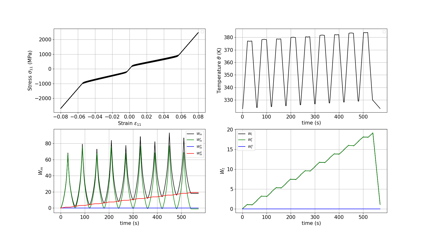
Plotting the results
We plot the stress-strain curve, the temperature evolution, the mechanical work terms and the thermal work terms for the SMA thermomechanical response.
fig = plt.figure()
outputfile_macro = os.path.join(path_results, "results_THERM_SMAUT_global-0.txt")

# Get the data
e11, e22, e33, e12, e13, e23, s11, s22, s33, s12, s13, s23 = np.loadtxt(
    outputfile_macro,
    usecols=(8, 9, 10, 11, 12, 13, 14, 15, 16, 17, 18, 19),
    unpack=True,
)
time, T, Q, r = np.loadtxt(outputfile_macro, usecols=(4, 5, 6, 7), unpack=True)
Wm, Wm_r, Wm_ir, Wm_d, Wt, Wt_r, Wt_ir = np.loadtxt(
    outputfile_macro, usecols=(20, 21, 22, 23, 24, 25, 26), unpack=True
)

# Stress vs Strain
ax = fig.add_subplot(2, 2, 1)
plt.grid(True)
plt.tick_params(axis="both", which="major", labelsize=15)
plt.xlabel(r"Strain $\varepsilon_{11}$", size=15)
plt.ylabel(r"Stress $\sigma_{11}$ (MPa)", size=15)
plt.plot(e11, s11, c="black")
plt.legend(loc="best")

# Temperature vs Time
ax = fig.add_subplot(2, 2, 2)
plt.grid(True)
plt.tick_params(axis="both", which="major", labelsize=15)
plt.xlabel("time (s)", size=15)
plt.ylabel(r"Temperature $\theta$ (K)", size=15)
plt.plot(time, T, c="black")
plt.legend(loc="best")

# Mechanical work vs Time
ax = fig.add_subplot(2, 2, 3)
plt.grid(True)
plt.tick_params(axis="both", which="major", labelsize=15)
plt.xlabel("time (s)", size=15)
plt.ylabel(r"$W_m$", size=15)
plt.plot(time, Wm, c="black", label=r"$W_m$")
plt.plot(time, Wm_r, c="green", label=r"$W_m^r$")
plt.plot(time, Wm_ir, c="blue", label=r"$W_m^{ir}$")
plt.plot(time, Wm_d, c="red", label=r"$W_m^d$")
plt.legend(loc="best")

# Thermal work vs Time
ax = fig.add_subplot(2, 2, 4)
plt.grid(True)
plt.tick_params(axis="both", which="major", labelsize=15)
plt.xlabel("time (s)", size=15)
plt.ylabel(r"$W_t$", size=15)
plt.plot(time, Wt, c="black", label=r"$W_t$")
plt.plot(time, Wt_r, c="green", label=r"$W_t^r$")
plt.plot(time, Wt_ir, c="blue", label=r"$W_t^{ir}$")
plt.legend(loc="best")

plt.show()
/home/runner/work/simcoon/simcoon/examples/thermomechanical/SMA_T.py:153: UserWarning: No artists with labels found to put in legend.  Note that artists whose label start with an underscore are ignored when legend() is called with no argument.
  plt.legend(loc="best")
/home/runner/work/simcoon/simcoon/examples/thermomechanical/SMA_T.py:162: UserWarning: No artists with labels found to put in legend.  Note that artists whose label start with an underscore are ignored when legend() is called with no argument.
  plt.legend(loc="best")
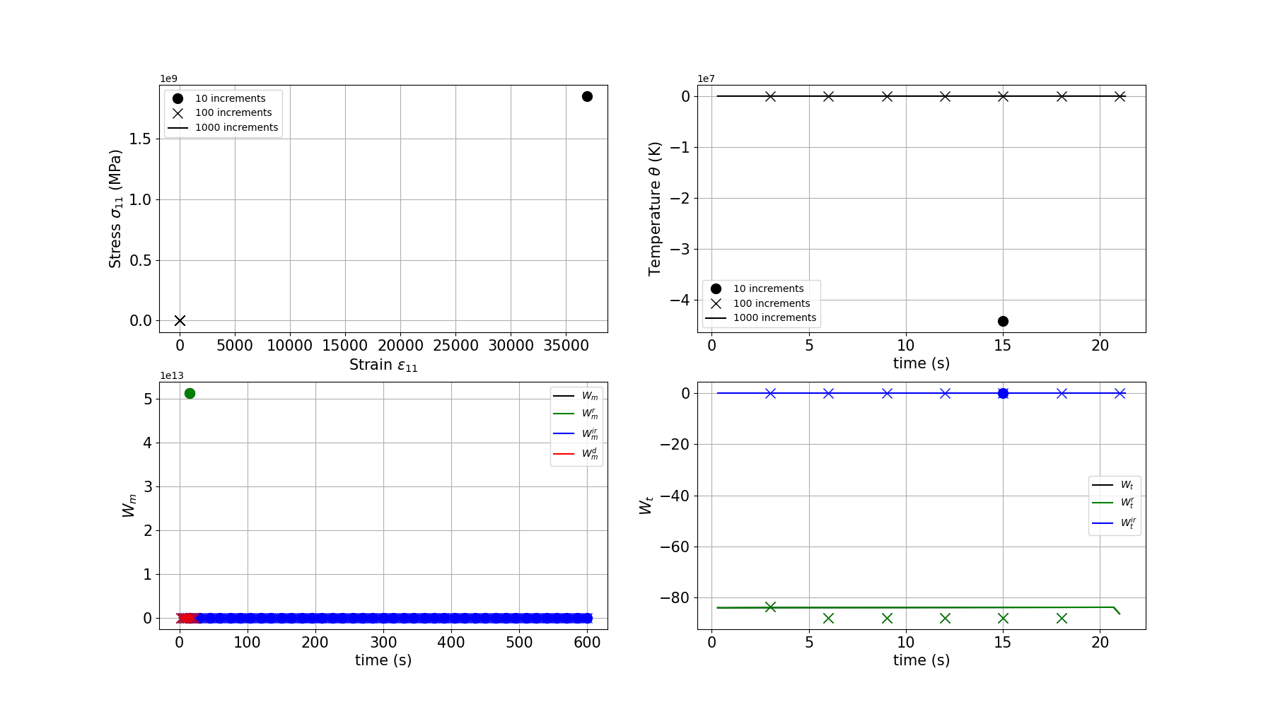
Increment size effect
Here we test the effect of the increment size on the results.
increments = [10, 100, 1000]
outputfile_globals = {}

for inc in increments:
    pathfile = f"THERM_SMAUT_path_{inc}.txt"
    outputfile = f"results_THERM_SMAUT_{inc}.txt"
    sim.solver(
        umat_name,
        props,
        nstatev,
        psi_rve,
        theta_rve,
        phi_rve,
        solver_type,
        corate_type,
        path_data,
        path_results,
        pathfile,
        outputfile,
    )
    outputfile_globals[inc] = f"results_THERM_SMAUT_{inc}_global-0.txt"

# Load data for each increment
data = []
for inc in increments:
    path = os.path.join(path_results, outputfile_globals[inc])
    e11, e22, e33, e12, e13, e23, s11, s22, s33, s12, s13, s23 = np.loadtxt(
        path, usecols=range(8, 20), unpack=True
    )
    time, T, Q, r = np.loadtxt(path, usecols=range(4, 8), unpack=True)
    Wm, Wm_r, Wm_ir, Wm_d, Wt, Wt_r, Wt_ir = np.loadtxt(
        path, usecols=range(20, 27), unpack=True
    )
    data.append(
        {
            "e11": e11, "s11": s11, "time": time, "T": T,
            "Wm": Wm, "Wm_r": Wm_r, "Wm_ir": Wm_ir, "Wm_d": Wm_d,
            "Wt": Wt, "Wt_r": Wt_r, "Wt_ir": Wt_ir,
        }
    )
Plotting the increment size comparison
fig = plt.figure()

markers = ["o", "x", None]
labels = ["10 increments", "100 increments", "1000 increments"]

# Stress vs Strain
ax = fig.add_subplot(2, 2, 1)
plt.grid(True)
plt.tick_params(axis="both", which="major", labelsize=15)
plt.xlabel(r"Strain $\varepsilon_{11}$", size=15)
plt.ylabel(r"Stress $\sigma_{11}$ (MPa)", size=15)
for i, d in enumerate(data):
    if markers[i] is not None:
        plt.plot(d["e11"], d["s11"], linestyle="None", marker=markers[i],
                 color="black", markersize=10, label=labels[i])
    else:
        plt.plot(d["e11"], d["s11"], c="black", label=labels[i])
plt.legend(loc="best")

# Temperature vs Time
ax = fig.add_subplot(2, 2, 2)
plt.grid(True)
plt.tick_params(axis="both", which="major", labelsize=15)
plt.xlabel("time (s)", size=15)
plt.ylabel(r"Temperature $\theta$ (K)", size=15)
for i, d in enumerate(data):
    if markers[i] is not None:
        plt.plot(d["time"], d["T"], linestyle="None", marker=markers[i],
                 color="black", markersize=10, label=labels[i])
    else:
        plt.plot(d["time"], d["T"], c="black", label=labels[i])
plt.legend(loc="best")

# Mechanical work vs Time
ax = fig.add_subplot(2, 2, 3)
plt.grid(True)
plt.tick_params(axis="both", which="major", labelsize=15)
plt.xlabel("time (s)", size=15)
plt.ylabel(r"$W_m$", size=15)
work_colors = ["black", "green", "blue", "red"]
work_keys = ["Wm", "Wm_r", "Wm_ir", "Wm_d"]
work_labels = [r"$W_m$", r"$W_m^r$", r"$W_m^{ir}$", r"$W_m^d$"]
for i, d in enumerate(data):
    for j, (wk, wc, wl) in enumerate(zip(work_keys, work_colors, work_labels)):
        if markers[i] is not None:
            plt.plot(d["time"], d[wk], linestyle="None", marker=markers[i],
                     color=wc, markersize=10)
        else:
            plt.plot(d["time"], d[wk], c=wc, label=wl)
plt.legend(loc="best")

# Thermal work vs Time
ax = fig.add_subplot(2, 2, 4)
plt.grid(True)
plt.tick_params(axis="both", which="major", labelsize=15)
plt.xlabel("time (s)", size=15)
plt.ylabel(r"$W_t$", size=15)
therm_keys = ["Wt", "Wt_r", "Wt_ir"]
therm_labels = [r"$W_t$", r"$W_t^r$", r"$W_t^{ir}$"]
therm_colors = ["black", "green", "blue"]
for i, d in enumerate(data):
    for j, (wk, wc, wl) in enumerate(zip(therm_keys, therm_colors, therm_labels)):
        if markers[i] is not None:
            plt.plot(d["time"], d[wk], linestyle="None", marker=markers[i],
                     color=wc, markersize=10)
        else:
            plt.plot(d["time"], d[wk], c=wc, label=wl)
plt.legend(loc="best")

plt.show()
Total running time of the script: (0 minutes 2.296 seconds)