Note
Go to the end to download the full example code.
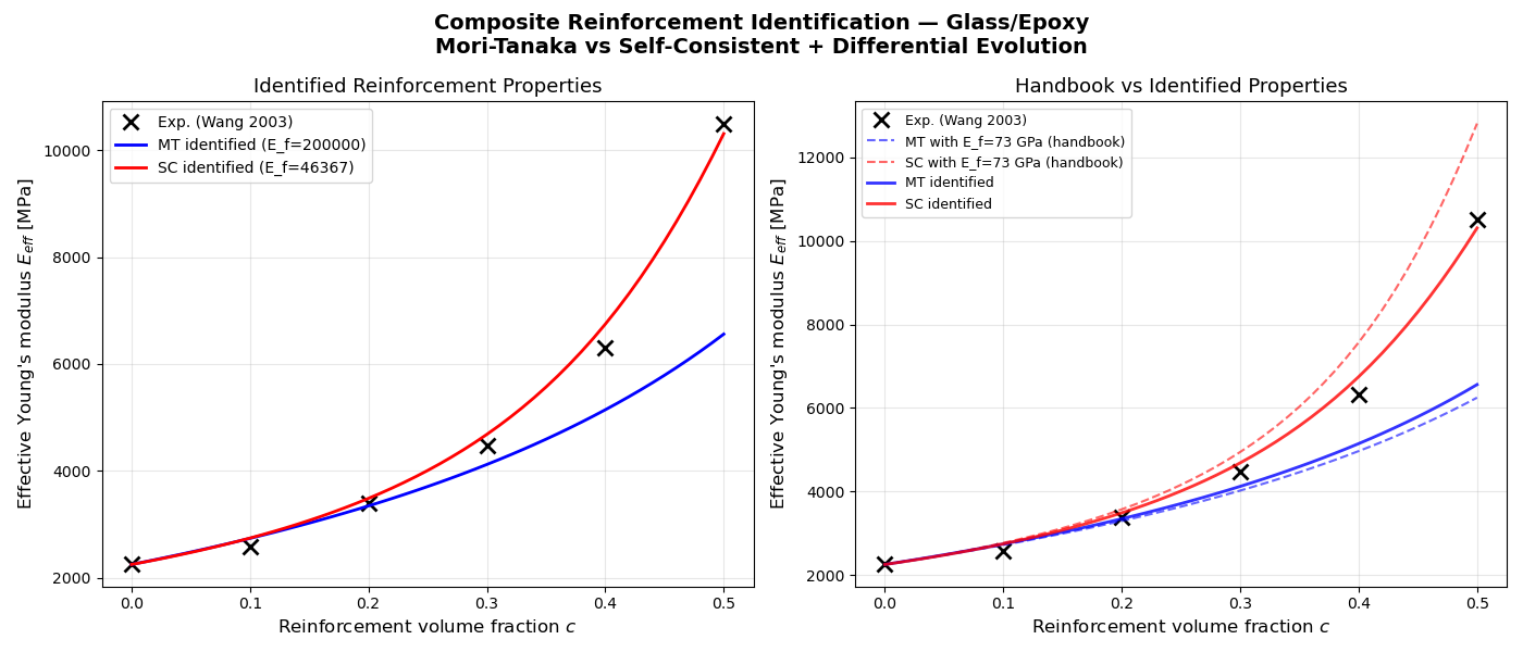
Composite Parameter Identification using Mori-Tanaka and Self-Consistent
This example demonstrates inverse identification of reinforcement elastic properties in a two-phase composite material. Given experimental effective Young’s modulus data at various volume fractions (Wang 2003), we identify the Young’s modulus and Poisson’s ratio of the reinforcement phase.
Two micromechanical schemes are compared:
Mori-Tanaka (
MIMTN): accurate at low-to-moderate volume fractionsSelf-Consistent (
MISCN): better at high volume fractions (c > 0.3)
Forward model: simcoon mean-field homogenization (L_eff)
Optimization: scipy.optimize.differential_evolution (global optimizer)
Key system: simcoon Parameter for generic file templating
import numpy as np
import matplotlib.pyplot as plt
from scipy.optimize import differential_evolution
import simcoon as sim
from simcoon import parameter as par
import os
Problem Setup
We have a glass-particle / epoxy composite. The matrix properties are known:
\(E_m = 2250\) MPa, \(\\nu_m = 0.19\)
The reinforcement properties \((E_f, \\nu_f)\) are unknown and must be identified from experimental effective Young’s modulus measurements at several volume fractions.
Key System: simcoon’s key system allows parameters to be injected into
any input file via alphanumeric placeholders (e.g., @2p). This makes the
identification workflow generic and applicable to any simulation tool
(simcoon solver, Mori-Tanaka, fedoo FE, etc.).
def load_experimental_data(filepath):
    """Load experimental E_eff vs volume fraction data."""
    data = np.loadtxt(filepath)
    return data[:, 0], data[:, 1]
Forward Model
For each set of candidate properties \((E_f, \\nu_f)\), we compute the
effective Young’s modulus at all experimental volume fractions using simcoon’s
L_eff function.
def compute_E_eff(
    E_f, nu_f, concentrations, umat_name, param_list, path_keys, path_data,
    props_composite,
):
    """
    Compute effective Young's modulus at given volume fractions.

    Parameters
    ----------
    E_f : float
        Reinforcement Young's modulus [MPa]
    nu_f : float
        Reinforcement Poisson's ratio [-]
    concentrations : array-like
        Volume fractions of reinforcement
    umat_name : str
        Micromechanical scheme ("MIMTN" or "MISCN")
    param_list : list of Parameter
        Parameter objects with keys for file templating
    path_keys : str
        Path to template files
    path_data : str
        Path to working data directory (must be "data" relative to cwd)
    props_composite : numpy.ndarray
        Composite definition array [nphases, num_file, int1, int2, n_matrix]

    Returns
    -------
    numpy.ndarray
        Effective Young's modulus at each volume fraction [MPa]
    """
    E_eff = np.zeros(len(concentrations))

    for i, c in enumerate(concentrations):
        param_list[0].value = 1.0 - c
        param_list[1].value = c
        param_list[2].value = E_f
        param_list[3].value = nu_f

        par.copy_parameters(param_list, path_keys, path_data)
        par.apply_parameters(param_list, path_data)

        L = sim.L_eff(umat_name, props_composite, 0, 0.0, 0.0, 0.0)
        iso_props = sim.L_iso_props(L).flatten()
        E_eff[i] = iso_props[0]

    return E_eff


def cost_function(
    params_opt, c_exp, E_exp, umat_name, param_list, path_keys, path_data,
    props_composite,
):
    """MSE cost function for reinforcement property identification."""
    E_f, nu_f = params_opt
    try:
        E_pred = compute_E_eff(
            E_f, nu_f, c_exp, umat_name, param_list, path_keys, path_data,
            props_composite,
        )
        return np.mean((E_pred - E_exp) ** 2)
    except Exception:
        return 1e12


def identify_reinforcement(
    c_exp, E_exp, umat_name, param_list, path_keys, path_data,
    props_composite, bounds, verbose=True,
):
    """
    Identify reinforcement properties using differential evolution.

    Returns
    -------
    dict
        Identified parameters and optimization result
    """
    if verbose:
        print(f"\n{'=' * 60}")
        print(f"  Identification with {umat_name}")
        print(f"{'=' * 60}")

    result = differential_evolution(
        cost_function,
        bounds=bounds,
        args=(c_exp, E_exp, umat_name, param_list, path_keys, path_data,
              props_composite),
        strategy="best1bin",
        maxiter=200,
        popsize=15,
        tol=1e-8,
        mutation=(0.5, 1.0),
        recombination=0.7,
        seed=42,
        polish=True,
        disp=verbose,
    )

    E_f_opt, nu_f_opt = result.x
    if verbose:
        print(f"\n  E_f  = {E_f_opt:.0f} MPa")
        print(f"  nu_f = {nu_f_opt:.3f}")
        print(f"  MSE  = {result.fun:.2e} MPa^2")

    return {
        "E_f": E_f_opt,
        "nu_f": nu_f_opt,
        "mse": result.fun,
        "result": result,
        "umat_name": umat_name,
    }
Main Execution
We compare two identification strategies:
Mori-Tanaka (
MIMTN): dilute approximation, best for c < 30%Self-Consistent (
MISCN): accounts for percolation, better at high c
At high volume fractions (c = 0.5), Mori-Tanaka underestimates stiffness and compensates by overestimating \(E_f\). Self-Consistent gives more physically meaningful identified properties.
if __name__ == "__main__":

    # -----------------------------------------------------------------
    # Change to example directory (L_eff reads from data/ in cwd)
    # -----------------------------------------------------------------
    try:
        script_dir = os.path.dirname(os.path.abspath(__file__))
    except NameError:
        script_dir = os.getcwd()
    os.chdir(script_dir)

    path_keys = "keys_ident"
    path_data = "data"

    # -----------------------------------------------------------------
    # Load experimental data (Wang 2003)
    # -----------------------------------------------------------------
    c_exp, E_exp = load_experimental_data("data/E_exp.txt")

    print("=" * 60)
    print(" COMPOSITE REINFORCEMENT IDENTIFICATION")
    print(" Glass/Epoxy — Mean-field + Differential Evolution")
    print("=" * 60)
    print(f"\nExperimental data (Wang 2003): {len(c_exp)} points")
    for c, E in zip(c_exp, E_exp):
        print(f"  c = {c:.1f}  ->  E_eff = {E:.0f} MPa")

    # -----------------------------------------------------------------
    # Load parameters (key system)
    # -----------------------------------------------------------------
    # Define parameters inline (no external file needed):
    #   @0p -> matrix concentration
    #   @1p -> reinforcement concentration
    #   @2p -> reinforcement E [MPa]
    #   @3p -> reinforcement nu
    param_list = [
        par.Parameter(0, bounds=(0.0, 1.0), key="@0p",
                      sim_input_files=["Nellipsoids0.dat"]),
        par.Parameter(1, bounds=(0.0, 1.0), key="@1p",
                      sim_input_files=["Nellipsoids0.dat"]),
        par.Parameter(2, bounds=(10000, 200000), key="@2p",
                      sim_input_files=["Nellipsoids0.dat"]),
        par.Parameter(3, bounds=(0.01, 0.45), key="@3p",
                      sim_input_files=["Nellipsoids0.dat"]),
    ]

    # Composite definition
    props_composite = np.array([2, 0, 50, 50, 0], dtype="float")

    # Bounds for identification (E_f, nu_f)
    bounds = [(10000, 200000), (0.01, 0.45)]

    # -----------------------------------------------------------------
    # Identification with Mori-Tanaka
    # -----------------------------------------------------------------
    result_MT = identify_reinforcement(
        c_exp, E_exp, "MIMTN", param_list, path_keys, path_data,
        props_composite, bounds,
    )

    # -----------------------------------------------------------------
    # Identification with Self-Consistent
    # -----------------------------------------------------------------
    result_SC = identify_reinforcement(
        c_exp, E_exp, "MISCN", param_list, path_keys, path_data,
        props_composite, bounds,
    )

    # -----------------------------------------------------------------
    # Summary
    # -----------------------------------------------------------------
    print(f"\n{'=' * 60}")
    print(f" SUMMARY")
    print(f"{'=' * 60}")
    print(f"  Reference glass: E_f ~ 73000 MPa, nu_f ~ 0.22")
    print(f"")
    print(f"  {'Scheme':<20} {'E_f [MPa]':>12} {'nu_f':>8} {'MSE':>14}")
    print(f"  {'-' * 56}")
    print(f"  {'Mori-Tanaka':<20} {result_MT['E_f']:>12.0f} "
          f"{result_MT['nu_f']:>8.3f} {result_MT['mse']:>14.2e}")
    print(f"  {'Self-Consistent':<20} {result_SC['E_f']:>12.0f} "
          f"{result_SC['nu_f']:>8.3f} {result_SC['mse']:>14.2e}")
    print()

    # Note on model limitations
    print("  Note: Mori-Tanaka underestimates stiffness at high volume")
    print("  fractions and compensates by overestimating E_f. Self-Consistent")
    print("  accounts for phase connectivity and gives more physically")
    print("  meaningful results for this dataset (c up to 50%).")

    # -----------------------------------------------------------------
    # Visualization
    # -----------------------------------------------------------------
    c_model = np.arange(0.0, 0.51, 0.01)

    E_MT = compute_E_eff(
        result_MT["E_f"], result_MT["nu_f"], c_model, "MIMTN",
        param_list, path_keys, path_data, props_composite,
    )
    E_SC = compute_E_eff(
        result_SC["E_f"], result_SC["nu_f"], c_model, "MISCN",
        param_list, path_keys, path_data, props_composite,
    )
    # Reference with handbook glass properties
    E_ref_MT = compute_E_eff(
        73000, 0.22, c_model, "MIMTN",
        param_list, path_keys, path_data, props_composite,
    )
    E_ref_SC = compute_E_eff(
        73000, 0.22, c_model, "MISCN",
        param_list, path_keys, path_data, props_composite,
    )

    fig, (ax1, ax2) = plt.subplots(1, 2, figsize=(14, 6))

    # Left: Identified fits
    ax1.plot(c_exp, E_exp, "kx", markersize=10, markeredgewidth=2,
             label="Exp. (Wang 2003)")
    ax1.plot(c_model, E_MT, "b-", linewidth=2,
             label=f"MT identified (E_f={result_MT['E_f']:.0f})")
    ax1.plot(c_model, E_SC, "r-", linewidth=2,
             label=f"SC identified (E_f={result_SC['E_f']:.0f})")
    ax1.set_xlabel("Reinforcement volume fraction $c$", fontsize=12)
    ax1.set_ylabel("Effective Young's modulus $E_{eff}$ [MPa]", fontsize=12)
    ax1.set_title("Identified Reinforcement Properties", fontsize=13)
    ax1.legend(fontsize=10)
    ax1.grid(True, alpha=0.3)

    # Right: Reference vs Identified
    ax2.plot(c_exp, E_exp, "kx", markersize=10, markeredgewidth=2,
             label="Exp. (Wang 2003)")
    ax2.plot(c_model, E_ref_MT, "b--", linewidth=1.5, alpha=0.6,
             label="MT with E_f=73 GPa (handbook)")
    ax2.plot(c_model, E_ref_SC, "r--", linewidth=1.5, alpha=0.6,
             label="SC with E_f=73 GPa (handbook)")
    ax2.plot(c_model, E_MT, "b-", linewidth=2, alpha=0.8,
             label="MT identified")
    ax2.plot(c_model, E_SC, "r-", linewidth=2, alpha=0.8,
             label="SC identified")
    ax2.set_xlabel("Reinforcement volume fraction $c$", fontsize=12)
    ax2.set_ylabel("Effective Young's modulus $E_{eff}$ [MPa]", fontsize=12)
    ax2.set_title("Handbook vs Identified Properties", fontsize=13)
    ax2.legend(fontsize=9)
    ax2.grid(True, alpha=0.3)

    fig.suptitle(
        "Composite Reinforcement Identification — Glass/Epoxy\n"
        "Mori-Tanaka vs Self-Consistent + Differential Evolution",
        fontsize=14, fontweight="bold",
    )
    plt.tight_layout()
    plt.show()
============================================================
 COMPOSITE REINFORCEMENT IDENTIFICATION
 Glass/Epoxy — Mean-field + Differential Evolution
============================================================

Experimental data (Wang 2003): 6 points
  c = 0.0  ->  E_eff = 2250 MPa
  c = 0.1  ->  E_eff = 2580 MPa
  c = 0.2  ->  E_eff = 3390 MPa
  c = 0.3  ->  E_eff = 4480 MPa
  c = 0.4  ->  E_eff = 6310 MPa
  c = 0.5  ->  E_eff = 10500 MPa

============================================================
  Identification with MIMTN
============================================================
differential_evolution step 1: f(x)= 2845441.8584308363
differential_evolution step 2: f(x)= 2845441.8584308363
differential_evolution step 3: f(x)= 2844384.527162666
differential_evolution step 4: f(x)= 2843372.44679017
differential_evolution step 5: f(x)= 2843130.1492564585
differential_evolution step 6: f(x)= 2842473.3377612284
differential_evolution step 7: f(x)= 2842473.3377612284
differential_evolution step 8: f(x)= 2841803.683566658
differential_evolution step 9: f(x)= 2841691.1728336983
differential_evolution step 10: f(x)= 2841691.1728336983
differential_evolution step 11: f(x)= 2841647.8003525925
differential_evolution step 12: f(x)= 2841602.746182008
differential_evolution step 13: f(x)= 2841453.417909387
differential_evolution step 14: f(x)= 2841453.417909387
differential_evolution step 15: f(x)= 2841453.417909387
differential_evolution step 16: f(x)= 2841453.417909387
differential_evolution step 17: f(x)= 2841419.1478061355
differential_evolution step 18: f(x)= 2841401.2186515722
differential_evolution step 19: f(x)= 2841401.2186515722
differential_evolution step 20: f(x)= 2841401.2186515722
differential_evolution step 21: f(x)= 2841401.2186515722
differential_evolution step 22: f(x)= 2841401.2186515722
differential_evolution step 23: f(x)= 2841401.2186515722
differential_evolution step 24: f(x)= 2841396.1084521133
differential_evolution step 25: f(x)= 2841396.1084521133
differential_evolution step 26: f(x)= 2841396.1084521133
differential_evolution step 27: f(x)= 2841393.3240744397
differential_evolution step 28: f(x)= 2841393.3240744397
differential_evolution step 29: f(x)= 2841393.3240744397
differential_evolution step 30: f(x)= 2841391.396678291
differential_evolution step 31: f(x)= 2841391.396678291
differential_evolution step 32: f(x)= 2841391.396678291
differential_evolution step 33: f(x)= 2841391.396678291
differential_evolution step 34: f(x)= 2841391.1774388435
differential_evolution step 35: f(x)= 2841390.819151416
differential_evolution step 36: f(x)= 2841390.2110353014
differential_evolution step 37: f(x)= 2841390.2110353014
differential_evolution step 38: f(x)= 2841390.2110353014
differential_evolution step 39: f(x)= 2841390.2110353014
differential_evolution step 40: f(x)= 2841390.2110353014
differential_evolution step 41: f(x)= 2841390.2110353014
differential_evolution step 42: f(x)= 2841390.2110353014
differential_evolution step 43: f(x)= 2841390.161741854
differential_evolution step 44: f(x)= 2841390.101437967
differential_evolution step 45: f(x)= 2841390.101437967
differential_evolution step 46: f(x)= 2841390.101437967
differential_evolution step 47: f(x)= 2841390.101437967
differential_evolution step 48: f(x)= 2841390.101437967
differential_evolution step 49: f(x)= 2841390.078150217
differential_evolution step 50: f(x)= 2841390.07126537
differential_evolution step 51: f(x)= 2841390.07126537
differential_evolution step 52: f(x)= 2841390.065127143
differential_evolution step 53: f(x)= 2841390.0629338934
differential_evolution step 54: f(x)= 2841390.0629338934
differential_evolution step 55: f(x)= 2841390.0629338934
differential_evolution step 56: f(x)= 2841390.060185104
Polishing solution with 'L-BFGS-B'

  E_f  = 200000 MPa
  nu_f = 0.450
  MSE  = 2.84e+06 MPa^2

============================================================
  Identification with MISCN
============================================================
differential_evolution step 1: f(x)= 54451.33263124695
differential_evolution step 2: f(x)= 52713.18502556835
differential_evolution step 3: f(x)= 52250.08051017501
differential_evolution step 4: f(x)= 52250.08051017501
differential_evolution step 5: f(x)= 51026.38861423012
differential_evolution step 6: f(x)= 50844.44748894559
differential_evolution step 7: f(x)= 50844.44748894559
differential_evolution step 8: f(x)= 50844.44748894559
differential_evolution step 9: f(x)= 50784.99401241427
differential_evolution step 10: f(x)= 50638.777388705355
differential_evolution step 11: f(x)= 50638.777388705355
differential_evolution step 12: f(x)= 50638.777388705355
differential_evolution step 13: f(x)= 50638.777388705355
differential_evolution step 14: f(x)= 50623.994479305074
differential_evolution step 15: f(x)= 50623.783592824555
differential_evolution step 16: f(x)= 50590.65814852624
differential_evolution step 17: f(x)= 50590.65814852624
differential_evolution step 18: f(x)= 50588.314183930845
differential_evolution step 19: f(x)= 50584.761535897684
differential_evolution step 20: f(x)= 50584.761535897684
differential_evolution step 21: f(x)= 50583.00679534065
differential_evolution step 22: f(x)= 50583.00679534065
differential_evolution step 23: f(x)= 50582.404035831416
differential_evolution step 24: f(x)= 50582.404035831416
differential_evolution step 25: f(x)= 50582.404035831416
differential_evolution step 26: f(x)= 50582.16590752159
differential_evolution step 27: f(x)= 50582.11894011469
differential_evolution step 28: f(x)= 50581.99120108114
differential_evolution step 29: f(x)= 50581.99120108114
differential_evolution step 30: f(x)= 50581.88523979694
differential_evolution step 31: f(x)= 50581.88523979694
differential_evolution step 32: f(x)= 50581.88523979694
differential_evolution step 33: f(x)= 50581.88523979694
differential_evolution step 34: f(x)= 50581.88523979694
differential_evolution step 35: f(x)= 50581.88523979694
differential_evolution step 36: f(x)= 50581.88523979694
differential_evolution step 37: f(x)= 50581.88523979694
differential_evolution step 38: f(x)= 50581.88147021726
differential_evolution step 39: f(x)= 50581.88147021726
differential_evolution step 40: f(x)= 50581.88147021726
differential_evolution step 41: f(x)= 50581.88121183913
differential_evolution step 42: f(x)= 50581.88104237749
differential_evolution step 43: f(x)= 50581.88085197378
differential_evolution step 44: f(x)= 50581.880180304695
differential_evolution step 45: f(x)= 50581.880180304695
differential_evolution step 46: f(x)= 50581.88017582471
differential_evolution step 47: f(x)= 50581.88017582471
differential_evolution step 48: f(x)= 50581.88017482083
Polishing solution with 'L-BFGS-B'

  E_f  = 46367 MPa
  nu_f = 0.010
  MSE  = 5.06e+04 MPa^2

============================================================
 SUMMARY
============================================================
  Reference glass: E_f ~ 73000 MPa, nu_f ~ 0.22

  Scheme                  E_f [MPa]     nu_f            MSE
  --------------------------------------------------------
  Mori-Tanaka                200000    0.450       2.84e+06
  Self-Consistent             46367    0.010       5.06e+04

  Note: Mori-Tanaka underestimates stiffness at high volume
  fractions and compensates by overestimating E_f. Self-Consistent
  accounts for phase connectivity and gives more physically
  meaningful results for this dataset (c up to 50%).
Total running time of the script: (2 minutes 40.451 seconds)