Plasticity with Chaboche Hardening Example

import os
import numpy as np
import matplotlib.pyplot as plt
import simcoon as sim

plt.rcParams["figure.figsize"] = (18, 10)

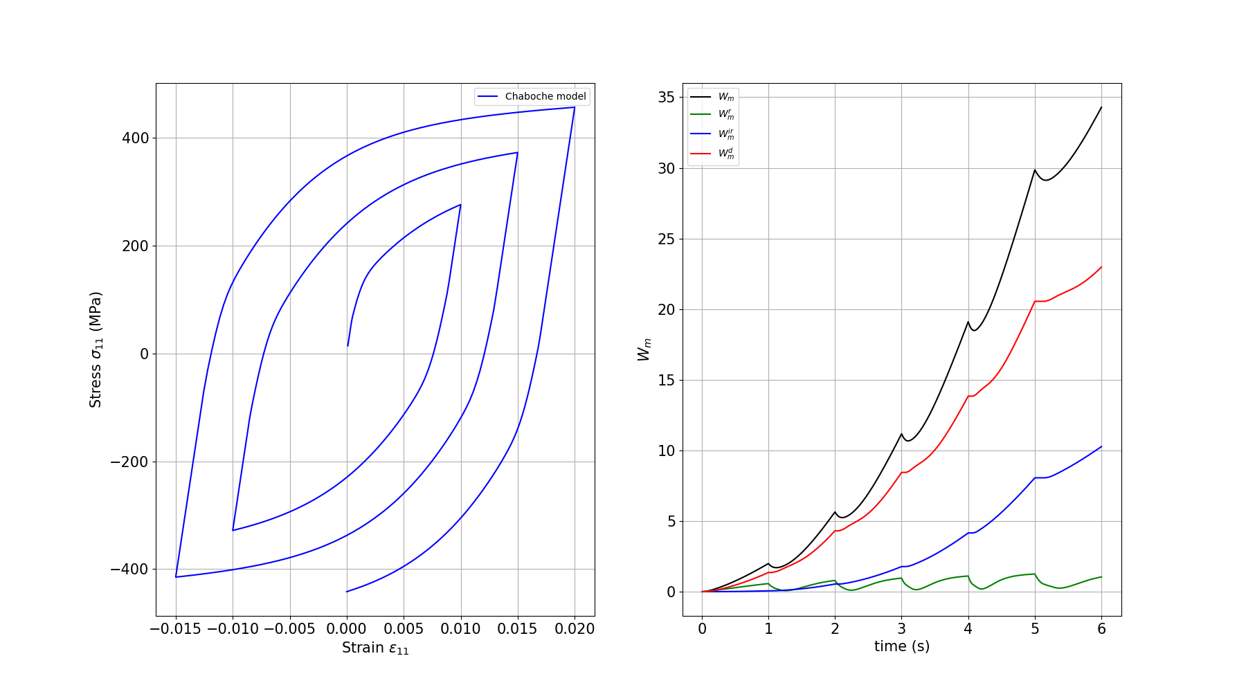
The Chaboche plasticity model combines isotropic and kinematic hardening. This model is particularly suited for cyclic loading applications where the Bauschinger effect is important.

Ten parameters are required:

1. The Young modulus \(E\)

2. The Poisson ratio \(\nu\)

3. The coefficient of thermal expansion \(\alpha\)

4. The initial yield stress \(\sigma_Y\)

5. The isotropic hardening saturation value \(Q\)

6. The isotropic hardening rate \(b\)

7. The first kinematic hardening modulus \(C_1\)

8. The first kinematic hardening rate \(D_1\)

9. The second kinematic hardening modulus \(C_2\)

10. The second kinematic hardening rate \(D_2\)

The constitutive law is given by:

\[\begin{split}{\sigma}_{ij} & = L_{ijkl}\left({\varepsilon}^{\textrm{tot}}_{kl}-\alpha_{kl}\left(T-T^{\textrm{ref}}\right)-{\varepsilon}^{\textrm{p}}_{kl}\right) \\ \dot{\varepsilon}^{\textrm{p}}_{ij} & =\dot{p}\Lambda_{ij}, \quad \Lambda_{ij}=\frac{3}{2}\frac{\sigma'_{ij} - X_{ij}}{\overline{\sigma} - X} \\ \dot{X}_{ij} & = \sum_{k} \frac{2}{3} C_k \dot{\varepsilon}^{\textrm{p}}_{ij} - D_k X^{(k)}_{ij} \dot{p} \\ \dot{R} & = b(Q - R)\dot{p} \\ \Phi & =\overline{\sigma - X}-\sigma_{Y}-R\leq 0\end{split}\]

where \(X_{ij}\) is the kinematic hardening (back stress) tensor and \(R\) is the isotropic hardening variable.

umat_name = "EPCHA"  # 5 character code for Chaboche plasticity
nstatev = 33  # Number of internal variables

# Material parameters
E = 140000.0  # Young's modulus (MPa)
nu = 0.3  # Poisson ratio
alpha = 1.0e-6  # Thermal expansion coefficient
sigma_Y = 62.859017  # Initial yield stress (MPa)
Q = 416.004456  # Isotropic hardening saturation
b = 4.788635  # Isotropic hardening rate
C_1 = 30382.293921  # First kinematic hardening modulus
D_1 = 172.425687  # First kinematic hardening rate
C_2 = 195142.490843  # Second kinematic hardening modulus
D_2 = 3012.614659  # Second kinematic hardening rate

psi_rve = 0.0
theta_rve = 0.0
phi_rve = 0.0
solver_type = 0
corate_type = 1

props = np.array([E, nu, alpha, sigma_Y, Q, b, C_1, D_1, C_2, D_2])

path_data = "../data"
pathfile = "EPCHA_path.json"

The loading path is read in Python and the simulation runs in memory: no result file is written, and the histories come back as component-first arrays.

blocks, T_init, _ = sim.solver.load_path_json(os.path.join(path_data, pathfile))

res = sim.solver.solve(
    blocks,
    umat_name,
    props,
    nstatev,
    T_init=T_init,
    solver_type=solver_type,
    corate=corate_type,
    orientation=(psi_rve, theta_rve, phi_rve),
)

Plotting the results

We plot the stress-strain hysteresis loop which shows the cyclic behavior including the Bauschinger effect from kinematic hardening.

e11, e22, e33, e12, e13, e23 = res["Strain"]
s11, s22, s33, s12, s13, s23 = res["Stress"]
time, T = res["Time"], res["Temp"]
Wm, Wm_r, Wm_ir, Wm_d = res["Wm"]

fig = plt.figure()

# First subplot: Stress vs Strain (hysteresis loop)
ax1 = fig.add_subplot(1, 2, 1)
plt.grid(True)
plt.tick_params(axis="both", which="major", labelsize=15)
plt.xlabel(r"Strain $\varepsilon_{11}$", size=15)
plt.ylabel(r"Stress $\sigma_{11}$ (MPa)", size=15)
plt.plot(e11, s11, c="blue", label="Chaboche model")
plt.legend(loc="best")

# Second subplot: Work terms vs Time
ax2 = fig.add_subplot(1, 2, 2)
plt.grid(True)
plt.tick_params(axis="both", which="major", labelsize=15)
plt.xlabel("time (s)", size=15)
plt.ylabel(r"$W_m$", size=15)
plt.plot(time, Wm, c="black", label=r"$W_m$")
plt.plot(time, Wm_r, c="green", label=r"$W_m^r$")
plt.plot(time, Wm_ir, c="blue", label=r"$W_m^{ir}$")
plt.plot(time, Wm_d, c="red", label=r"$W_m^d$")
plt.legend(loc="best")

plt.show()