Modular UMAT under Finite Strain — Hencky Hyperelasto-Plasticity

Runs the same composable "MODUL" material as MODUL.py, but under finite strain (NLGEOM): control type 3 drives the logarithmic strain / Kirchhoff stress conjugate pair, and the solver kinematics hand the model the log strain of the actual deformation gradient. The elasticity block then acts as a Hencky stored-energy function of ln V and the plasticity mechanism rides additively on that measure — a genuine hyperelasto-plastic model.

This holds only when the accumulated corotational strain is exactly ln V, which is the log_R corate: corate_type = 3 is REQUIRED for MODUL under NLGEOM and any other corate raises a RuntimeError (a Jaumann- or Green-Naghdi-integrated model would be hypoelastic and dissipate spuriously in closed cycles).

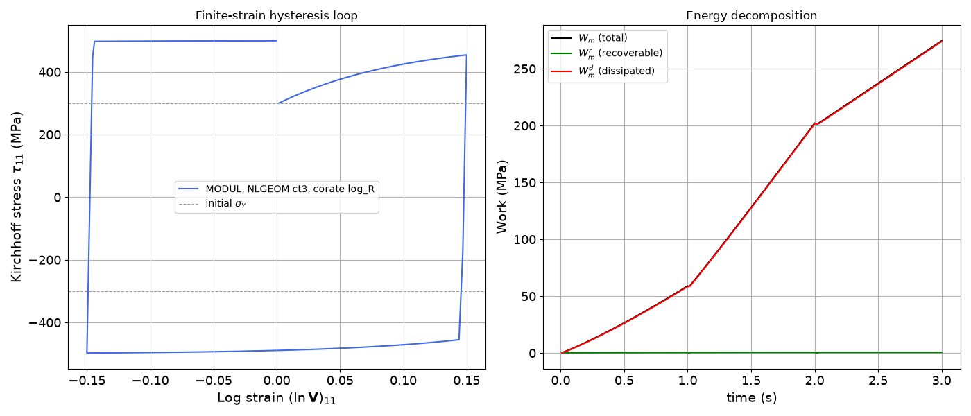
The path file drives a log-strain cycle +15% / -15% / 0 — genuinely finite stretches (lambda from 0.86 to 1.16) — exposing the elasto-plastic hysteresis loop in the (ln V, tau) work-conjugate plane.

import os
import numpy as np
import matplotlib.pyplot as plt
import simcoon as sim
from simcoon.modular import (
    ModularMaterial,
    IsotropicElasticity,
    Plasticity,
    VonMisesYield,
    VoceHardening,
)

plt.rcParams["figure.figsize"] = (14, 6)

1. Compose the constitutive model

Same composition as MODUL.py: isotropic elasticity (“Enu”: C1 = E, C2 = nu) + von Mises yield + Voce isotropic hardening.

mat = ModularMaterial(
    elasticity=IsotropicElasticity(
        C1=210000.0, C2=0.3, alpha=1.2e-5, convention="Enu"
    ),
    mechanisms=[
        Plasticity(
            sigma_Y=300.0,
            yield_criterion=VonMisesYield(),
            isotropic_hardening=VoceHardening(Q=200.0, b=10.0),
        ),
    ],
)

print(mat.summary())

ModularMaterial:
  Elasticity: IsotropicElasticity
    C1=210000.0, C2=0.3, alpha=1.2e-05 [ENU]
  Mechanisms (1):
    [0] Plasticity
        sigma_Y=300.0
        yield: VonMisesYield
        iso_hard: VoceHardening
        kin_hard: NoKinematicHardening
  nprops=15, nstatev=8

2. Run the solver under NLGEOM

The path file sets Control_type(NLGEOM) = 3 (log strain / Kirchhoff stress). corate_type = 3 (log_R) is mandatory for MODUL under finite strain.

corate_type = 3  # log_R — the only hyper/hypo-consistent corate for MODUL

os.makedirs("results", exist_ok=True)

sim._core.solver(
    mat.umat_name,
    mat.props,
    mat.nstatev,
    0.0,            # psi_rve
    0.0,            # theta_rve
    0.0,            # phi_rve
    0,              # solver_type
    corate_type,
    "../data",
    "results",
    "MODUL_finite_path.txt",
    "results_MODUL_finite.txt",
)

3. Plot the response

The default output (no output.dat) reports Green-Lagrange strain and Cauchy stress. This path is rotation-free with fixed principal axes, so the conversion to the work-conjugate (ln V, Kirchhoff) pair of the model is exact: per normal component lambda_i^2 = 1 + 2 E_ii, (ln V)_ii = ln(lambda_i), and tau = J * sigma with J = lambda_1 lambda_2 lambda_3.

outputfile_macro = os.path.join("results", "results_MODUL_finite_global-0.txt")

time, e11_GL, e22_GL, e33_GL, s11_cauchy, Wm, Wm_r, Wm_d = np.loadtxt(
    outputfile_macro, usecols=(4, 8, 9, 10, 14, 20, 21, 23), unpack=True
)

e11 = 0.5 * np.log(1.0 + 2.0 * e11_GL)             # log strain (ln V)_11
J = np.sqrt((1 + 2 * e11_GL) * (1 + 2 * e22_GL) * (1 + 2 * e33_GL))
s11 = J * s11_cauchy                               # Kirchhoff stress tau_11

fig = plt.figure()

ax1 = fig.add_subplot(1, 2, 1)
plt.grid(True)
plt.tick_params(axis="both", which="major", labelsize=13)
plt.xlabel(r"Log strain $(\ln \mathbf{V})_{11}$", size=14)
plt.ylabel(r"Kirchhoff stress $\tau_{11}$ (MPa)", size=14)
plt.plot(e11, s11, c="royalblue", lw=1.5,
         label="MODUL, NLGEOM ct3, corate log_R")
plt.axhline(y=300.0, color="0.6", linestyle="--", lw=0.8,
            label=r"initial $\sigma_Y$")
plt.axhline(y=-300.0, color="0.6", linestyle="--", lw=0.8)
plt.legend(loc="best")
plt.title("Finite-strain hysteresis loop")

ax2 = fig.add_subplot(1, 2, 2)
plt.grid(True)
plt.tick_params(axis="both", which="major", labelsize=13)
plt.xlabel("time (s)", size=14)
plt.ylabel("Work (MPa)", size=14)
plt.plot(time, Wm, c="black", label=r"$W_m$ (total)")
plt.plot(time, Wm_r, c="green", label=r"$W_m^r$ (recoverable)")
plt.plot(time, Wm_d, c="red", label=r"$W_m^d$ (dissipated)")
plt.legend(loc="best")
plt.title("Energy decomposition")

plt.tight_layout()
plt.savefig("MODUL_finite_stress_strain.png", dpi=120)
plt.show()