Modular UMAT Example — Composable Elasto-Plasticity

Demonstrates the simcoon.modular high-level Python interface that composes a constitutive model declaratively and runs it through the standard sim.solver load-path driver. The C++ ModularUMAT infrastructure (ElasticityModule, YieldCriterion, hardening, …) is internal — the user only builds a ModularMaterial and hands its .props / .nstatev to the "MODUL" UMAT code registered in simcoon’s UMAT table.

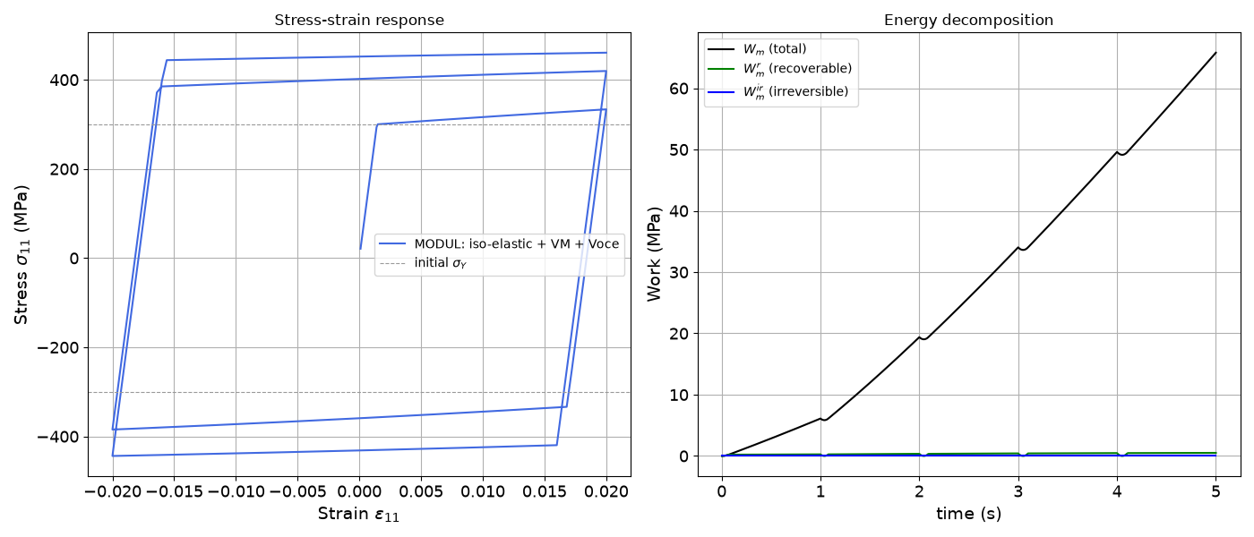
The path file applies a monotonic tensile ramp to 2% strain, then two strain-controlled cycles between -2% and +2%, exposing isotropic-hardening growth and the initial yield plateau.

import os
import numpy as np
import matplotlib.pyplot as plt
import simcoon as sim
from simcoon.modular import (
    ModularMaterial,
    IsotropicElasticity,
    Plasticity,
    VonMisesYield,
    VoceHardening,
)

plt.rcParams["figure.figsize"] = (14, 6)

1. Compose the constitutive model

Isotropic elasticity + von Mises yield + Voce isotropic hardening. Parameters: E=210 GPa, nu=0.3, sigma_Y=300 MPa, Q=200 MPa, b=10.

The elastic constants C1/C2 are ordinal slots whose meaning is fixed by the convention argument — here "Enu" (C1 = E, C2 = nu). Other parameterizations (“Kmu”, “lambdamu”, …) are accepted as well.

mat = ModularMaterial(
    elasticity=IsotropicElasticity(
        C1=210000.0, C2=0.3, alpha=1.2e-5, convention="Enu"
    ),
    mechanisms=[
        Plasticity(
            sigma_Y=300.0,
            yield_criterion=VonMisesYield(),
            isotropic_hardening=VoceHardening(Q=200.0, b=10.0),
        ),
    ],
)

print(mat.summary())

ModularMaterial:
  Elasticity: IsotropicElasticity
    C1=210000.0, C2=0.3, alpha=1.2e-05 [ENU]
  Mechanisms (1):
    [0] Plasticity
        sigma_Y=300.0
        yield: VonMisesYield
        iso_hard: VoceHardening
        kin_hard: NoKinematicHardening
  nprops=15, nstatev=8

2. Run the solver

mat.umat_name is "MODUL", the UMAT code registered at umat_smart.cpp:316 (id 200). mat.props serializes the composition into the flat array that the C++ umat_modular deserializes.

umat_name = mat.umat_name
props = mat.props
nstatev = mat.nstatev

psi_rve = 0.0
theta_rve = 0.0
phi_rve = 0.0
solver_type = 0
corate_type = 1

path_data = "../data"
path_results = "results"
pathfile = "MODUL_path.txt"
outputfile = "results_MODUL.txt"

os.makedirs(path_results, exist_ok=True)

sim._core.solver(
    umat_name,
    props,
    nstatev,
    psi_rve,
    theta_rve,
    phi_rve,
    solver_type,
    corate_type,
    path_data,
    path_results,
    pathfile,
    outputfile,
)

3. Plot the stress-strain curve

outputfile_macro = os.path.join(path_results, "results_MODUL_global-0.txt")

e11, e22, e33, e12, e13, e23, s11, s22, s33, s12, s13, s23 = np.loadtxt(
    outputfile_macro,
    usecols=(8, 9, 10, 11, 12, 13, 14, 15, 16, 17, 18, 19),
    unpack=True,
)
time, T, Q_out, r = np.loadtxt(outputfile_macro, usecols=(4, 5, 6, 7), unpack=True)
Wm, Wm_r, Wm_ir, Wm_d = np.loadtxt(
    outputfile_macro, usecols=(20, 21, 22, 23), unpack=True
)

fig = plt.figure()

# Stress-strain curve
ax1 = fig.add_subplot(1, 2, 1)
plt.grid(True)
plt.tick_params(axis="both", which="major", labelsize=13)
plt.xlabel(r"Strain $\varepsilon_{11}$", size=14)
plt.ylabel(r"Stress $\sigma_{11}$ (MPa)", size=14)
plt.plot(e11, s11, c="royalblue", lw=1.5, label="MODUL: iso-elastic + VM + Voce")
plt.axhline(y=300.0, color="0.6", linestyle="--", lw=0.8, label=r"initial $\sigma_Y$")
plt.axhline(y=-300.0, color="0.6", linestyle="--", lw=0.8)
plt.legend(loc="best")
plt.title("Stress-strain response")

# Work terms vs time
ax2 = fig.add_subplot(1, 2, 2)
plt.grid(True)
plt.tick_params(axis="both", which="major", labelsize=13)
plt.xlabel("time (s)", size=14)
plt.ylabel("Work (MPa)", size=14)
plt.plot(time, Wm, c="black", label=r"$W_m$ (total)")
plt.plot(time, Wm_r, c="green", label=r"$W_m^r$ (recoverable)")
plt.plot(time, Wm_ir, c="blue", label=r"$W_m^{ir}$ (irreversible)")
plt.legend(loc="best")
plt.title("Energy decomposition")

plt.tight_layout()
plt.savefig("MODUL_stress_strain.png", dpi=120)
plt.show()