Chaboche Cyclic Plasticity Identification

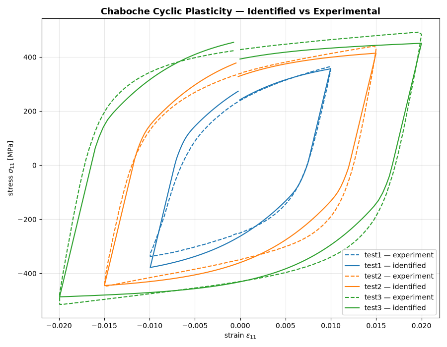
Identify 7 elasto-plastic Chaboche parameters from 3 cyclic uniaxial tests.

Material model: EPCHA UMAT — linear elasticity + Voce isotropic hardening + two non-linear kinematic backstresses.

Symbol	Parameter	Bounds
sigmaY	initial yield	50 – 300 MPa
Q, b	Voce isotropic	100 – 10000 MPa, 0.01 – 10
C_1, D_1	1st backstress	1e3 – 1e5 MPa, 10 – 1000
C_2, D_2	2nd backstress	1e4 – 1e6 MPa, 10 – 10000

Fixed: \(E = 140000\) MPa, \(\nu = 0.3\), \(\alpha = 10^{-6}\).

The three tests are cyclic strain-controlled tensile experiments at increasing amplitudes (~1%, ~1.5%, ~2%). Each one needs a pre-cycling stage so the numerical model arrives at the comparison window with realistic accumulated backstress, then an initial-state alignment so it starts at the same residual strain as the experiment, then a replay of the experimental loading path. This is encoded in three blocks of the structured path_id_N.txt config file:

1. Block 1 (mode 1, linear) — virtual pre-cycle (±1%, ±1.5%, ±2%)

2. Block 2 (mode 1, linear) — set initial residual strain (first row of exp)

3. Block 3 (mode 3, tab file) — replay tab_file_N.txt

The path_id_N.txt and tab_file_N.txt files are provided in data/ because they are tricky to construct manually. When feature/python_solver lands, this scaffolding will be replaced by Python helpers that build steps and tab files programmatically from the experimental data.

Forward model: simcoon.solver() (UMAT material-point integrator). Optimization: simcoon.identification() (wraps differential_evolution). Cost: nmse_per_response — normalises each test’s stress column by its own sum of squares, balancing the three tests despite different stress magnitudes.

============================================================
 CHABOCHE CYCLIC PLASTICITY IDENTIFICATION
 7 params from 3 cyclic tests, NMSE-per-response cost
============================================================
  test1: path_id_1.txt + tab_file_1.txt vs exp_file_1.txt  (201 pts)
  test2: path_id_2.txt + tab_file_15.txt vs exp_file_15.txt  (201 pts)
  test3: path_id_3.txt + tab_file_2.txt vs exp_file_2.txt  (200 pts)

============================================================
 IDENTIFIED PARAMETERS
============================================================
  sigmaY   =      100.952    (bounds (50, 300))
  Q        =      322.569    (bounds (100, 10000))
  b        =        6.592    (bounds (0.01, 10.0))
  C_1      =    28439.293    (bounds (1000, 100000))
  D_1      =      161.459    (bounds (10, 1000))
  C_2      =   130459.212    (bounds (10000, 1000000.0))
  D_2      =     3681.648    (bounds (10, 10000))

  Final cost (NMSE/response) = 8.2397e-03

import os
import numpy as np
import matplotlib.pyplot as plt
import simcoon as sim
from simcoon.parameter import Parameter
from simcoon.identify import identification, calc_cost


# ---------------------------------------------------------------------------
# Test catalogue — file naming mirrors the legacy ``03 - Identification``
# layout (numbering is intentional: 1, 1.5, 2 strain amplitudes).
# ---------------------------------------------------------------------------
TESTS = [
    # name      path file         tab file           exp file
    ("test1", "path_id_1.txt", "tab_file_1.txt",  "exp_file_1.txt"),
    ("test2", "path_id_2.txt", "tab_file_15.txt", "exp_file_15.txt"),
    ("test3", "path_id_3.txt", "tab_file_2.txt",  "exp_file_2.txt"),
]

UMAT_NAME = "EPCHA"
NSTATEV = 33
SOLVER_TYPE = 0
CORATE_TYPE = 2

# Fixed (not identified)
E_FIXED = 140000.0
NU_FIXED = 0.3
ALPHA_FIXED = 1.0e-6

# Identified — order matches the EPCHA props vector after E, nu, alpha.
PARAMS = [
    Parameter(1, bounds=(50,    300),    key="@1p"),  # sigmaY
    Parameter(2, bounds=(100,   10000),  key="@2p"),  # Q
    Parameter(3, bounds=(0.01,  10.0),   key="@3p"),  # b
    Parameter(4, bounds=(1000,  100000), key="@4p"),  # C_1
    Parameter(5, bounds=(10,    1000),   key="@5p"),  # D_1
    Parameter(6, bounds=(10000, 1.0e6),  key="@6p"),  # C_2
    Parameter(7, bounds=(10,    10000),  key="@7p"),  # D_2
]
PARAM_NAMES = ["sigmaY", "Q", "b", "C_1", "D_1", "C_2", "D_2"]

# σ11 lives at column 14 of the simcoon ``_global-0.txt`` output
# (cols 8–13 = strain Voigt, 14–19 = stress Voigt).
SIGMA11_COL = 14


def build_props(x):
    """Assemble the EPCHA props vector from the optimizer's parameter array."""
    return np.array([E_FIXED, NU_FIXED, ALPHA_FIXED, *x])


def run_one_test(props, pathfile, outputfile, path_data, path_results):
    """Run one solver call and return the predicted σ11 trajectory."""
    sim.solver(
        UMAT_NAME, props, NSTATEV,
        0.0, 0.0, 0.0,                  # psi, theta, phi
        SOLVER_TYPE, CORATE_TYPE,
        path_data, path_results,
        pathfile, outputfile,
    )
    base = outputfile[:-4] if outputfile.endswith(".txt") else outputfile
    out = np.loadtxt(os.path.join(path_results, f"{base}_global-0.txt"))
    return out[:, SIGMA11_COL]


def cost(x, exp_stresses, path_data, path_results):
    """NMSE-per-response cost across the three tests."""
    props = build_props(x)
    y_num = []
    for name, pathfile, _tab, _exp in TESTS:
        try:
            sigma11 = run_one_test(
                props, pathfile, f"sim_{name}.txt", path_data, path_results
            )
        except Exception:
            return 1e12
        y_num.append(sigma11.reshape(-1, 1))
    return calc_cost(exp_stresses, y_num, metric="nmse_per_response")


def main():
    # sim.solver reads/writes relative to cwd
    try:
        script_dir = os.path.dirname(os.path.abspath(__file__))
    except NameError:
        script_dir = os.getcwd()
    os.chdir(script_dir)

    path_data = "data"
    path_results = "results"
    path_exp = "exp_data"
    os.makedirs(path_results, exist_ok=True)

    # Experimental σ11 — exp file columns: incr, time, strain, stress
    exp_stresses = []
    for _, _, _, expfile in TESTS:
        exp = np.loadtxt(os.path.join(path_exp, expfile))
        exp_stresses.append(exp[:, 3].reshape(-1, 1))

    print("=" * 60)
    print(" CHABOCHE CYCLIC PLASTICITY IDENTIFICATION")
    print(" 7 params from 3 cyclic tests, NMSE-per-response cost")
    print("=" * 60)
    for i, (name, pathfile, tab, expfile) in enumerate(TESTS):
        print(f"  {name}: {pathfile} + {tab} vs {expfile}  "
              f"({len(exp_stresses[i])} pts)")

    # Gallery budget (~1-2 min). Bump popsize/maxiter for tighter fits.
    result = identification(
        cost, PARAMS,
        args=(exp_stresses, path_data, path_results),
        seed=42,
        popsize=15, maxiter=80, tol=1e-6,
        disp=False,
    )

    print()
    print("=" * 60)
    print(" IDENTIFIED PARAMETERS")
    print("=" * 60)
    for n, p in zip(PARAM_NAMES, PARAMS):
        print(f"  {n:8s} = {p.value:>12.3f}    (bounds {p.bounds})")
    print(f"\n  Final cost (NMSE/response) = {result.fun:.4e}")

    # All three tests on one plot — dashed = experiment, solid = identified
    fig, ax = plt.subplots(figsize=(9, 7))
    final_props = build_props(np.array([p.value for p in PARAMS]))
    colors = ["tab:blue", "tab:orange", "tab:green"]
    for (name, pathfile, _tab, expfile), color in zip(TESTS, colors):
        exp = np.loadtxt(os.path.join(path_exp, expfile))
        sigma_num = run_one_test(
            final_props, pathfile, f"sim_{name}_final.txt",
            path_data, path_results,
        )
        ax.plot(exp[:, 2], exp[:, 3], color=color, linestyle="--",
                linewidth=1.5, label=f"{name} — experiment")
        ax.plot(exp[:, 2], sigma_num, color=color, linestyle="-",
                linewidth=1.5, label=f"{name} — identified")
    ax.set_xlabel(r"strain $\varepsilon_{11}$")
    ax.set_ylabel(r"stress $\sigma_{11}$ [MPa]")
    ax.set_title("Chaboche Cyclic Plasticity — Identified vs Experimental",
                 fontsize=13, fontweight="bold")
    ax.grid(True, alpha=0.3)
    ax.legend(loc="best", framealpha=0.9)
    plt.tight_layout()
    plt.show()


if __name__ == "__main__":
    main()