Transversely isotropic elasticity (thermomechanical)

import numpy as np
import simcoon as sim
import matplotlib.pyplot as plt
import os

plt.rcParams["figure.figsize"] = (18, 10)

In thermoelastic transversely isotropic materials, the following parameters are required:

The density \(\rho\)
The specific heat \(c_p\)
The axis of transverse isotropy (1, 2, or 3)
The longitudinal Young modulus \(E_L\)
The transverse Young modulus \(E_T\)
The Poisson ratio \(\nu_{TL}\)
The Poisson ratio \(\nu_{TT}\)
The shear modulus \(G_{LT}\)
The longitudinal thermal expansion coefficient \(\alpha_L\)
The transverse thermal expansion coefficient \(\alpha_T\)

The elastic stiffness tensor for a transversely isotropic material with axis 1 as the symmetry axis is written in the Voigt notation formalism as:

\[\begin{split}\mathbf{L} = \begin{pmatrix} L_{1111} & L_{1122} & L_{1122} & 0 & 0 & 0 \\ L_{1122} & L_{2222} & L_{2233} & 0 & 0 & 0 \\ L_{1122} & L_{2233} & L_{2222} & 0 & 0 & 0 \\ 0 & 0 & 0 & L_{1212} & 0 & 0 \\ 0 & 0 & 0 & 0 & L_{1212} & 0 \\ 0 & 0 & 0 & 0 & 0 & L_{2323} \end{pmatrix}\end{split}\]

The thermal expansion tensor is:

\[\begin{split}\boldsymbol{\alpha} = \begin{pmatrix} \alpha_L & 0 & 0 \\ 0 & \alpha_T & 0 \\ 0 & 0 & \alpha_T \end{pmatrix}\end{split}\]

umat_name = "ELIST"  # 5 character code for transversely isotropic elastic subroutine
nstatev = 1  # Number of internal variables

# Material parameters
rho = 4.4  # Density
c_p = 0.656  # Specific heat capacity
axis = 1  # Symmetry axis
E_L = 4500.0  # Longitudinal Young's modulus (MPa)
E_T = 2300.0  # Transverse Young's modulus (MPa)
nu_TL = 0.05  # Poisson ratio (transverse-longitudinal)
nu_TT = 0.3  # Poisson ratio (transverse-transverse)
G_LT = 2700.0  # Shear modulus (longitudinal-transverse) (MPa)
alpha_L = 1.0e-5  # Thermal expansion (longitudinal)
alpha_T = 2.5e-5  # Thermal expansion (transverse)

psi_rve = 0.0
theta_rve = 0.0
phi_rve = 0.0
solver_type = 0
corate_type = 2

props = np.array([rho, c_p, axis, E_L, E_T, nu_TL, nu_TT, G_LT, alpha_L, alpha_T])

path_data = "../data"
path_results = "results"

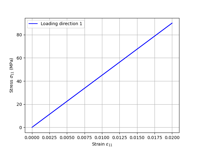
Loading in direction 1

First we apply a uniaxial stress loading along direction 1 (the symmetry axis).

pathfile = "THERM_ELISO_path_1.txt"
outputfile_1 = "results_THERM_ELIST_1.txt"

sim.solver(
    umat_name,
    props,
    nstatev,
    psi_rve,
    theta_rve,
    phi_rve,
    solver_type,
    corate_type,
    path_data,
    path_results,
    pathfile,
    outputfile_1,
)

outputfile_macro_1 = os.path.join(path_results, "results_THERM_ELIST_1_global-0.txt")

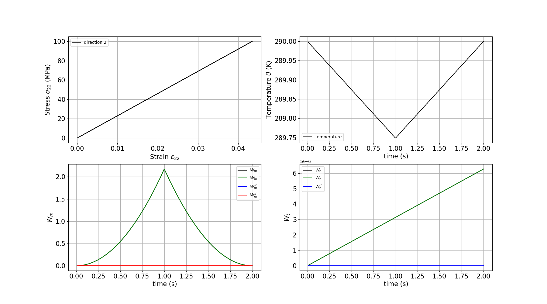
Loading in direction 2

Then we apply a uniaxial stress loading along direction 2 (the transverse direction).

pathfile = "THERM_ELISO_path_2.txt"
outputfile_2 = "results_THERM_ELIST_2.txt"

sim.solver(
    umat_name,
    props,
    nstatev,
    psi_rve,
    theta_rve,
    phi_rve,
    solver_type,
    corate_type,
    path_data,
    path_results,
    pathfile,
    outputfile_2,
)

outputfile_macro_2 = os.path.join(path_results, "results_THERM_ELIST_2_global-0.txt")

Plotting the results – Loading direction 1

We plot the stress-strain curve, the temperature evolution, and the work terms for loading along direction 1.

fig = plt.figure()

# Get the data
e11, e22, e33, e12, e13, e23, s11, s22, s33, s12, s13, s23 = np.loadtxt(
    outputfile_macro_1,
    usecols=(8, 9, 10, 11, 12, 13, 14, 15, 16, 17, 18, 19),
    unpack=True,
)
time, T, Q, r = np.loadtxt(outputfile_macro_1, usecols=(4, 5, 6, 7), unpack=True)
Wm, Wm_r, Wm_ir, Wm_d, Wt, Wt_r, Wt_ir = np.loadtxt(
    outputfile_macro_1, usecols=(20, 21, 22, 23, 24, 25, 26), unpack=True
)

# Stress vs Strain
ax = fig.add_subplot(2, 2, 1)
plt.grid(True)
plt.tick_params(axis="both", which="major", labelsize=15)
plt.xlabel(r"Strain $\varepsilon_{11}$", size=15)
plt.ylabel(r"Stress $\sigma_{11}$ (MPa)", size=15)
plt.plot(e11, s11, c="black", label="direction 1")
plt.legend(loc="best")

# Temperature vs Time
ax = fig.add_subplot(2, 2, 2)
plt.grid(True)
plt.tick_params(axis="both", which="major", labelsize=15)
plt.xlabel("time (s)", size=15)
plt.ylabel(r"Temperature $\theta$ (K)", size=15)
plt.plot(time, T, c="black", label="temperature")
plt.legend(loc="best")

# Mechanical work vs Time
ax = fig.add_subplot(2, 2, 3)
plt.grid(True)
plt.tick_params(axis="both", which="major", labelsize=15)
plt.xlabel("time (s)", size=15)
plt.ylabel(r"$W_m$", size=15)
plt.plot(time, Wm, c="black", label=r"$W_m$")
plt.plot(time, Wm_r, c="green", label=r"$W_m^r$")
plt.plot(time, Wm_ir, c="blue", label=r"$W_m^{ir}$")
plt.plot(time, Wm_d, c="red", label=r"$W_m^d$")
plt.legend(loc="best")

# Thermal work vs Time
ax = fig.add_subplot(2, 2, 4)
plt.grid(True)
plt.tick_params(axis="both", which="major", labelsize=15)
plt.xlabel("time (s)", size=15)
plt.ylabel(r"$W_t$", size=15)
plt.plot(time, Wt, c="black", label=r"$W_t$")
plt.plot(time, Wt_r, c="green", label=r"$W_t^r$")
plt.plot(time, Wt_ir, c="blue", label=r"$W_t^{ir}$")
plt.legend(loc="best")

plt.show()

Plotting the results – Loading direction 2

We plot the stress-strain curve, the temperature evolution, and the work terms for loading along direction 2.

fig = plt.figure()

# Get the data
e11, e22, e33, e12, e13, e23, s11, s22, s33, s12, s13, s23 = np.loadtxt(
    outputfile_macro_2,
    usecols=(8, 9, 10, 11, 12, 13, 14, 15, 16, 17, 18, 19),
    unpack=True,
)
time, T, Q, r = np.loadtxt(outputfile_macro_2, usecols=(4, 5, 6, 7), unpack=True)
Wm, Wm_r, Wm_ir, Wm_d, Wt, Wt_r, Wt_ir = np.loadtxt(
    outputfile_macro_2, usecols=(20, 21, 22, 23, 24, 25, 26), unpack=True
)

# Stress vs Strain
ax = fig.add_subplot(2, 2, 1)
plt.grid(True)
plt.tick_params(axis="both", which="major", labelsize=15)
plt.xlabel(r"Strain $\varepsilon_{22}$", size=15)
plt.ylabel(r"Stress $\sigma_{22}$ (MPa)", size=15)
plt.plot(e22, s22, c="black", label="direction 2")
plt.legend(loc="best")

# Temperature vs Time
ax = fig.add_subplot(2, 2, 2)
plt.grid(True)
plt.tick_params(axis="both", which="major", labelsize=15)
plt.xlabel("time (s)", size=15)
plt.ylabel(r"Temperature $\theta$ (K)", size=15)
plt.plot(time, T, c="black", label="temperature")
plt.legend(loc="best")

# Mechanical work vs Time
ax = fig.add_subplot(2, 2, 3)
plt.grid(True)
plt.tick_params(axis="both", which="major", labelsize=15)
plt.xlabel("time (s)", size=15)
plt.ylabel(r"$W_m$", size=15)
plt.plot(time, Wm, c="black", label=r"$W_m$")
plt.plot(time, Wm_r, c="green", label=r"$W_m^r$")
plt.plot(time, Wm_ir, c="blue", label=r"$W_m^{ir}$")
plt.plot(time, Wm_d, c="red", label=r"$W_m^d$")
plt.legend(loc="best")

# Thermal work vs Time
ax = fig.add_subplot(2, 2, 4)
plt.grid(True)
plt.tick_params(axis="both", which="major", labelsize=15)
plt.xlabel("time (s)", size=15)
plt.ylabel(r"$W_t$", size=15)
plt.plot(time, Wt, c="black", label=r"$W_t$")
plt.plot(time, Wt_r, c="green", label=r"$W_t^r$")
plt.plot(time, Wt_ir, c="blue", label=r"$W_t^{ir}$")
plt.legend(loc="best")

plt.show()

Total running time of the script: (0 minutes 0.422 seconds)

Gallery generated by Sphinx-Gallery