Note
Go to the end to download the full example code.
Orthotropic elasticity (thermomechanical)
import numpy as np
import simcoon as sim
import matplotlib.pyplot as plt
import os

plt.rcParams["figure.figsize"] = (18, 10)
In thermoelastic orthotropic materials, there are three mutually perpendicular planes of symmetry. The following parameters are required:
The density \(\rho\)
The specific heat \(c_p\)
The Young modulus in direction 1: \(E_1\)
The Young modulus in direction 2: \(E_2\)
The Young modulus in direction 3: \(E_3\)
The Poisson ratio \(\nu_{12}\)
The Poisson ratio \(\nu_{13}\)
The Poisson ratio \(\nu_{23}\)
The shear modulus \(G_{12}\)
The shear modulus \(G_{13}\)
The shear modulus \(G_{23}\)
The coefficient of thermal expansion \(\alpha_1\)
The coefficient of thermal expansion \(\alpha_2\)
The coefficient of thermal expansion \(\alpha_3\)
The elastic stiffness tensor for an orthotropic material is written in the Voigt notation as:
The thermal expansion tensor is:
umat_name = "ELORT"  # 5 character code for orthotropic elastic subroutine
nstatev = 1  # Number of internal variables

# Material parameters
rho = 4.4  # Density
c_p = 0.656  # Specific heat capacity
E_1 = 4500.0  # Young's modulus in direction 1 (MPa)
E_2 = 2300.0  # Young's modulus in direction 2 (MPa)
E_3 = 2700.0  # Young's modulus in direction 3 (MPa)
nu_12 = 0.06  # Poisson ratio 12
nu_13 = 0.08  # Poisson ratio 13
nu_23 = 0.3  # Poisson ratio 23
G_12 = 2200.0  # Shear modulus 12 (MPa)
G_13 = 2100.0  # Shear modulus 13 (MPa)
G_23 = 2400.0  # Shear modulus 23 (MPa)
alpha_1 = 1.0e-5  # Thermal expansion in direction 1
alpha_2 = 2.5e-5  # Thermal expansion in direction 2
alpha_3 = 2.2e-5  # Thermal expansion in direction 3

psi_rve = 0.0
theta_rve = 0.0
phi_rve = 0.0
solver_type = 0
corate_type = 2

props = np.array(
    [rho, c_p, E_1, E_2, E_3, nu_12, nu_13, nu_23, G_12, G_13, G_23, alpha_1, alpha_2, alpha_3]
)

path_data = "../data"
path_results = "results"
Loading in direction 1
pathfile = "THERM_ELISO_path_1.txt"
outputfile_1 = "results_THERM_ELORT_1.txt"

sim.solver(
    umat_name,
    props,
    nstatev,
    psi_rve,
    theta_rve,
    phi_rve,
    solver_type,
    corate_type,
    path_data,
    path_results,
    pathfile,
    outputfile_1,
)

outputfile_macro_1 = os.path.join(path_results, "results_THERM_ELORT_1_global-0.txt")
Loading in direction 2
pathfile = "THERM_ELISO_path_2.txt"
outputfile_2 = "results_THERM_ELORT_2.txt"

sim.solver(
    umat_name,
    props,
    nstatev,
    psi_rve,
    theta_rve,
    phi_rve,
    solver_type,
    corate_type,
    path_data,
    path_results,
    pathfile,
    outputfile_2,
)

outputfile_macro_2 = os.path.join(path_results, "results_THERM_ELORT_2_global-0.txt")
Loading in direction 3
pathfile = "THERM_ELISO_path_3.txt"
outputfile_3 = "results_THERM_ELORT_3.txt"

sim.solver(
    umat_name,
    props,
    nstatev,
    psi_rve,
    theta_rve,
    phi_rve,
    solver_type,
    corate_type,
    path_data,
    path_results,
    pathfile,
    outputfile_3,
)

outputfile_macro_3 = os.path.join(path_results, "results_THERM_ELORT_3_global-0.txt")
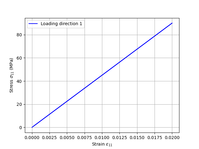
Plotting the results – Loading direction 1
fig = plt.figure()

e11, e22, e33, e12, e13, e23, s11, s22, s33, s12, s13, s23 = np.loadtxt(
    outputfile_macro_1,
    usecols=(8, 9, 10, 11, 12, 13, 14, 15, 16, 17, 18, 19),
    unpack=True,
)
time, T, Q, r = np.loadtxt(outputfile_macro_1, usecols=(4, 5, 6, 7), unpack=True)
Wm, Wm_r, Wm_ir, Wm_d, Wt, Wt_r, Wt_ir = np.loadtxt(
    outputfile_macro_1, usecols=(20, 21, 22, 23, 24, 25, 26), unpack=True
)

ax = fig.add_subplot(2, 2, 1)
plt.grid(True)
plt.tick_params(axis="both", which="major", labelsize=15)
plt.xlabel(r"Strain $\varepsilon_{11}$", size=15)
plt.ylabel(r"Stress $\sigma_{11}$ (MPa)", size=15)
plt.plot(e11, s11, c="black", label="direction 1")
plt.legend(loc="best")

ax = fig.add_subplot(2, 2, 2)
plt.grid(True)
plt.tick_params(axis="both", which="major", labelsize=15)
plt.xlabel("time (s)", size=15)
plt.ylabel(r"Temperature $\theta$ (K)", size=15)
plt.plot(time, T, c="black", label="temperature")
plt.legend(loc="best")

ax = fig.add_subplot(2, 2, 3)
plt.grid(True)
plt.tick_params(axis="both", which="major", labelsize=15)
plt.xlabel("time (s)", size=15)
plt.ylabel(r"$W_m$", size=15)
plt.plot(time, Wm, c="black", label=r"$W_m$")
plt.plot(time, Wm_r, c="green", label=r"$W_m^r$")
plt.plot(time, Wm_ir, c="blue", label=r"$W_m^{ir}$")
plt.plot(time, Wm_d, c="red", label=r"$W_m^d$")
plt.legend(loc="best")

ax = fig.add_subplot(2, 2, 4)
plt.grid(True)
plt.tick_params(axis="both", which="major", labelsize=15)
plt.xlabel("time (s)", size=15)
plt.ylabel(r"$W_t$", size=15)
plt.plot(time, Wt, c="black", label=r"$W_t$")
plt.plot(time, Wt_r, c="green", label=r"$W_t^r$")
plt.plot(time, Wt_ir, c="blue", label=r"$W_t^{ir}$")
plt.legend(loc="best")

plt.show()
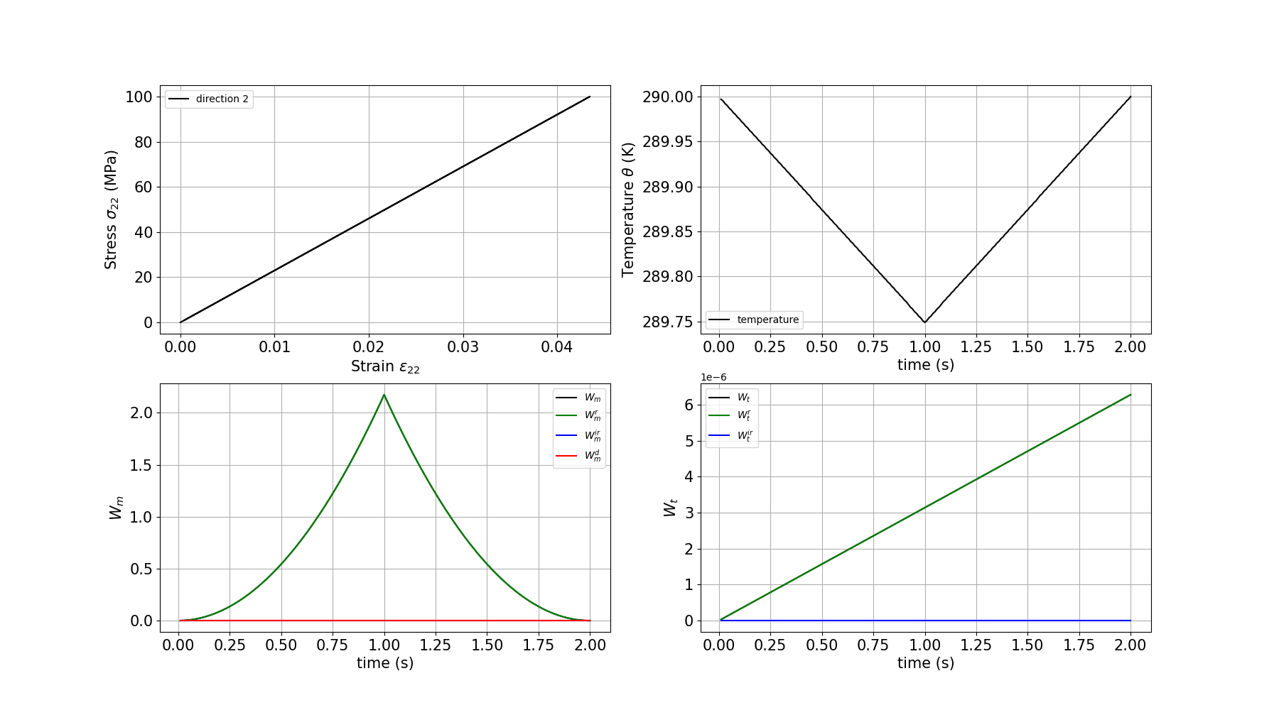
Plotting the results – Loading direction 2
fig = plt.figure()

e11, e22, e33, e12, e13, e23, s11, s22, s33, s12, s13, s23 = np.loadtxt(
    outputfile_macro_2,
    usecols=(8, 9, 10, 11, 12, 13, 14, 15, 16, 17, 18, 19),
    unpack=True,
)
time, T, Q, r = np.loadtxt(outputfile_macro_2, usecols=(4, 5, 6, 7), unpack=True)
Wm, Wm_r, Wm_ir, Wm_d, Wt, Wt_r, Wt_ir = np.loadtxt(
    outputfile_macro_2, usecols=(20, 21, 22, 23, 24, 25, 26), unpack=True
)

ax = fig.add_subplot(2, 2, 1)
plt.grid(True)
plt.tick_params(axis="both", which="major", labelsize=15)
plt.xlabel(r"Strain $\varepsilon_{22}$", size=15)
plt.ylabel(r"Stress $\sigma_{22}$ (MPa)", size=15)
plt.plot(e22, s22, c="black", label="direction 2")
plt.legend(loc="best")

ax = fig.add_subplot(2, 2, 2)
plt.grid(True)
plt.tick_params(axis="both", which="major", labelsize=15)
plt.xlabel("time (s)", size=15)
plt.ylabel(r"Temperature $\theta$ (K)", size=15)
plt.plot(time, T, c="black", label="temperature")
plt.legend(loc="best")

ax = fig.add_subplot(2, 2, 3)
plt.grid(True)
plt.tick_params(axis="both", which="major", labelsize=15)
plt.xlabel("time (s)", size=15)
plt.ylabel(r"$W_m$", size=15)
plt.plot(time, Wm, c="black", label=r"$W_m$")
plt.plot(time, Wm_r, c="green", label=r"$W_m^r$")
plt.plot(time, Wm_ir, c="blue", label=r"$W_m^{ir}$")
plt.plot(time, Wm_d, c="red", label=r"$W_m^d$")
plt.legend(loc="best")

ax = fig.add_subplot(2, 2, 4)
plt.grid(True)
plt.tick_params(axis="both", which="major", labelsize=15)
plt.xlabel("time (s)", size=15)
plt.ylabel(r"$W_t$", size=15)
plt.plot(time, Wt, c="black", label=r"$W_t$")
plt.plot(time, Wt_r, c="green", label=r"$W_t^r$")
plt.plot(time, Wt_ir, c="blue", label=r"$W_t^{ir}$")
plt.legend(loc="best")

plt.show()
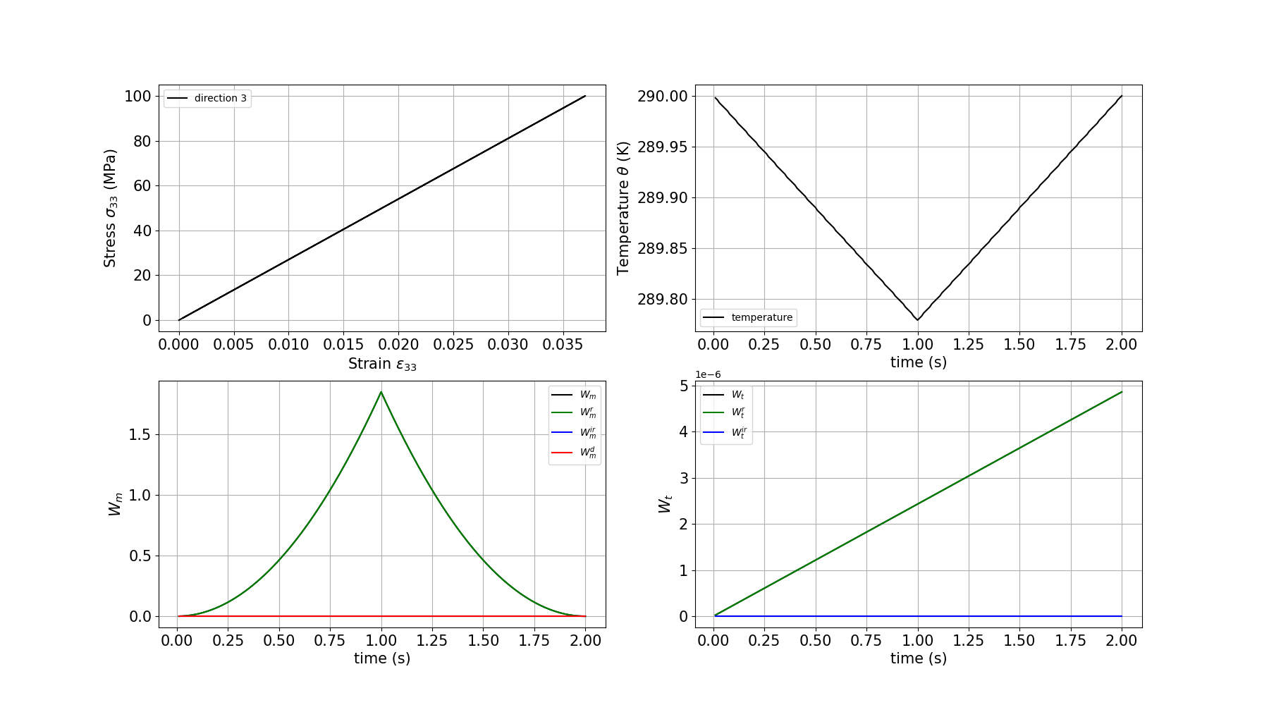
Plotting the results – Loading direction 3
fig = plt.figure()

e11, e22, e33, e12, e13, e23, s11, s22, s33, s12, s13, s23 = np.loadtxt(
    outputfile_macro_3,
    usecols=(8, 9, 10, 11, 12, 13, 14, 15, 16, 17, 18, 19),
    unpack=True,
)
time, T, Q, r = np.loadtxt(outputfile_macro_3, usecols=(4, 5, 6, 7), unpack=True)
Wm, Wm_r, Wm_ir, Wm_d, Wt, Wt_r, Wt_ir = np.loadtxt(
    outputfile_macro_3, usecols=(20, 21, 22, 23, 24, 25, 26), unpack=True
)

ax = fig.add_subplot(2, 2, 1)
plt.grid(True)
plt.tick_params(axis="both", which="major", labelsize=15)
plt.xlabel(r"Strain $\varepsilon_{33}$", size=15)
plt.ylabel(r"Stress $\sigma_{33}$ (MPa)", size=15)
plt.plot(e33, s33, c="black", label="direction 3")
plt.legend(loc="best")

ax = fig.add_subplot(2, 2, 2)
plt.grid(True)
plt.tick_params(axis="both", which="major", labelsize=15)
plt.xlabel("time (s)", size=15)
plt.ylabel(r"Temperature $\theta$ (K)", size=15)
plt.plot(time, T, c="black", label="temperature")
plt.legend(loc="best")

ax = fig.add_subplot(2, 2, 3)
plt.grid(True)
plt.tick_params(axis="both", which="major", labelsize=15)
plt.xlabel("time (s)", size=15)
plt.ylabel(r"$W_m$", size=15)
plt.plot(time, Wm, c="black", label=r"$W_m$")
plt.plot(time, Wm_r, c="green", label=r"$W_m^r$")
plt.plot(time, Wm_ir, c="blue", label=r"$W_m^{ir}$")
plt.plot(time, Wm_d, c="red", label=r"$W_m^d$")
plt.legend(loc="best")

ax = fig.add_subplot(2, 2, 4)
plt.grid(True)
plt.tick_params(axis="both", which="major", labelsize=15)
plt.xlabel("time (s)", size=15)
plt.ylabel(r"$W_t$", size=15)
plt.plot(time, Wt, c="black", label=r"$W_t$")
plt.plot(time, Wt_r, c="green", label=r"$W_t^r$")
plt.plot(time, Wt_ir, c="blue", label=r"$W_t^{ir}$")
plt.legend(loc="best")

plt.show()
Total running time of the script: (0 minutes 0.747 seconds)