Modular UMAT: Hyperelastic Block with Prony Branches (Finite-Strain Viscoelasticity)

Composes a "MODUL" material from a Yeoh hyperelastic block and a generalized-Maxwell viscoelastic mechanism (Prony branches), and drives it under finite strain (NLGEOM, control type "logarithmic", corate log_R): a rubber-like solid whose stiffness relaxes with time.

How the two compose. Under NLGEOM the solver hands the model the logarithmic strain ln V, the hyperelastic block is a stored-energy function of the elastic part ln V - eps_v (through b_el = exp(2 eps_el)), and each Prony branch is a Maxwell element living on that same logarithmic measure: branch i carries the stress L_i : (ln V - eps_v_i) and flows through its viscosity tensor H_i(etaB, etaS). The elasticity block therefore plays the instantaneous (glassy) role: at t = 0 the response is the Yeoh potential itself, and as the branches relax the stress drops toward a long-term response obtained by subtracting the branch strains through the ground-state compliance of the potential. That long-term response is not itself a hyperelastic potential, so this is not the classical rubber model of an equilibrium spring carrying Maxwell branches; it is the Hencky-space linear-viscoelastic overlay of the modular framework, exact in the small-strain limit and rate-consistent at large stretch.

Two consequences worth keeping in mind when calibrating:

• the branch moduli must stay below the ground-state modulus of the potential, sum_i E_i < E_0 with E_0 built from K = kappa and mu = 2 C10 (nothing validates this, and a violation gives a negative long-term stiffness);

• a branch is described by its modulus and viscosities, so a relaxation time tau is entered as etaS = tau * mu_i and etaB = tau * K_i.

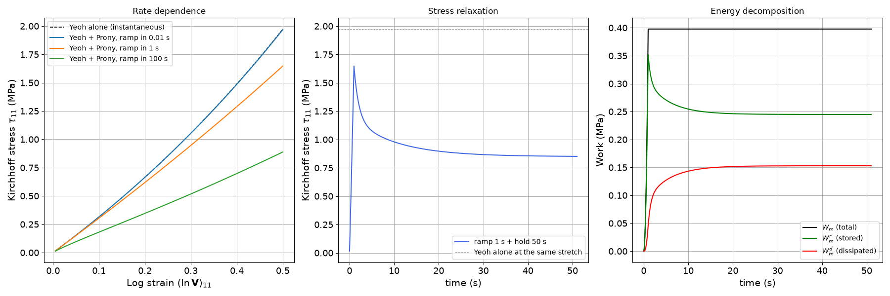
The script runs the same ramp to ln V = 0.5 (stretch 1.65) at three rates, bracketing the instantaneous (pure Yeoh) and the long-term responses, then a ramp-and-hold relaxation with its energy decomposition.

Both the material and the loading path are built in Python, and the results come back in memory.

import numpy as np
import matplotlib.pyplot as plt
from simcoon import solver
from simcoon.modular import ModularMaterial, YeohElasticity, Viscoelasticity

plt.rcParams["figure.figsize"] = (18, 6)

1. Compose the constitutive model

A Yeoh potential \(W = C_{10}(\bar I_1 - 3) + C_{20}(\bar I_1 - 3)^2 + C_{30}(\bar I_1 - 3)^3 + \kappa (J \ln J - J + 1)\) with a nearly incompressible bulk modulus, and two Prony branches with relaxation times of 1 s and 10 s. The branches are given as (E_i, nu_i, etaB_i, etaS_i); the helper below builds them from a modulus and a relaxation time.

C10, C20, C30, kappa = 0.5, -0.02, 0.002, 500.0     # MPa
mu0 = 2.0 * C10
E0 = 9.0 * kappa * mu0 / (3.0 * kappa + mu0)       # ground-state Young's modulus


def prony_branch(E, nu, tau):
    """(E, nu, etaB, etaS) for a Maxwell branch relaxing in ``tau`` seconds."""
    mu = E / (2.0 * (1.0 + nu))
    K = E / (3.0 * (1.0 - 2.0 * nu))
    return (E, nu, tau * K, tau * mu)


branches = (prony_branch(1.0, 0.49, 1.0), prony_branch(0.5, 0.49, 10.0))
assert sum(b[0] for b in branches) < E0, "branch moduli must stay below E_0"

yeoh = YeohElasticity(C10=C10, C20=C20, C30=C30, kappa=kappa)
mat = ModularMaterial(elasticity=yeoh, mechanisms=[Viscoelasticity(terms=branches)])
mat_inst = ModularMaterial(elasticity=yeoh)   # instantaneous response: pure Yeoh

print(mat.summary())
print(f"ground-state E_0 = {E0:.3f} MPa, long-term E_inf = "
      f"{E0 - sum(b[0] for b in branches):.3f} MPa")

ModularMaterial:
  Elasticity: YeohElasticity
    volumetric=log, C10=0.5, C20=-0.02, C30=0.002, kappa=500.0, alpha=0.0
  Mechanisms (1):
    [0] Viscoelasticity
        2 Prony terms (E_i, nu_i, etaB_i, etaS_i)
          [0] E=1.0, nu=0.49, etaB=16.666666666666654, etaS=0.33557046979865773
          [1] E=0.5, nu=0.49, etaB=83.33333333333327, etaS=1.6778523489932886
  nprops=20, nstatev=15
ground-state E_0 = 2.998 MPa, long-term E_inf = 1.498 MPa

2. Loading paths

Uniaxial tension in the log-strain / Kirchhoff-stress conjugate pair: the axial log strain is driven, the five other components are held stress-free.

uniaxial = ["strain"] + ["stress"] * 5


def ramp(eps, duration, ninc=100):
    return solver.StepMeca(control=uniaxial, value=[eps, 0, 0, 0, 0, 0],
                           time=duration, ninc=ninc, Dn_mini=1.0e-3)


def hold(eps, duration, ninc=200):
    return solver.StepMeca(control=uniaxial, value=[eps, 0, 0, 0, 0, 0],
                           time=duration, ninc=ninc)


def run(material, steps):
    return solver.solve(
        solver.Block(steps=steps, control_type="logarithmic"),
        material.umat_name, material.props, material.nstatev,
        corate="logarithmic_R",
    )


eps_max = 0.5                                      # ln V = 0.5, stretch 1.65

3. Rate sweep

The same ramp in 0.01 s (fast against both branches), 1 s and 100 s (slow against both), compared with the pure Yeoh block.

rates = {"0.01 s": 0.01, "1 s": 1.0, "100 s": 100.0}
sweep = {label: run(mat, [ramp(eps_max, t)]) for label, t in rates.items()}
inst = run(mat_inst, [ramp(eps_max, 1.0)])

4. Ramp and hold

Ramp to ln V = 0.5 in 1 s, then hold 50 s: the stress relaxes from the instantaneous level toward the long-term one.

relax = run(mat, [ramp(eps_max, 1.0), hold(eps_max, 50.0)])
tau11, t = relax["Kirchhoff"][0], relax["Time"]
Wm, Wm_r, _, Wm_d = relax["Wm"]
i_peak = int(np.argmin(np.abs(t - 1.0)))
print(f"relaxation: tau_11 = {tau11[i_peak]:.3f} MPa at the end of the ramp, "
      f"{tau11[-1]:.3f} MPa after {t[-1] - t[i_peak]:.0f} s of hold")

relaxation: tau_11 = 1.648 MPa at the end of the ramp, 0.851 MPa after 50 s of hold

5. Plot

fig = plt.figure()

ax1 = fig.add_subplot(1, 3, 1)
plt.grid(True)
plt.tick_params(axis="both", which="major", labelsize=13)
plt.xlabel(r"Log strain $(\ln \mathbf{V})_{11}$", size=14)
plt.ylabel(r"Kirchhoff stress $\tau_{11}$ (MPa)", size=14)
plt.plot(inst["LogStrain"][0], inst["Kirchhoff"][0], "k--", lw=1.2,
         label="Yeoh alone (instantaneous)")
for label, res in sweep.items():
    plt.plot(res["LogStrain"][0], res["Kirchhoff"][0], lw=1.5,
             label=f"Yeoh + Prony, ramp in {label}")
plt.legend(loc="best")
plt.title("Rate dependence")

ax2 = fig.add_subplot(1, 3, 2)
plt.grid(True)
plt.tick_params(axis="both", which="major", labelsize=13)
plt.xlabel("time (s)", size=14)
plt.ylabel(r"Kirchhoff stress $\tau_{11}$ (MPa)", size=14)
plt.plot(t, tau11, c="royalblue", lw=1.5, label="ramp 1 s + hold 50 s")
plt.axhline(y=inst["Kirchhoff"][0][-1], color="0.6", linestyle="--", lw=0.8,
            label="Yeoh alone at the same stretch")
plt.legend(loc="best")
plt.title("Stress relaxation")

ax3 = fig.add_subplot(1, 3, 3)
plt.grid(True)
plt.tick_params(axis="both", which="major", labelsize=13)
plt.xlabel("time (s)", size=14)
plt.ylabel("Work (MPa)", size=14)
plt.plot(t, Wm, c="black", label=r"$W_m$ (total)")
plt.plot(t, Wm_r, c="green", label=r"$W_m^r$ (stored)")
plt.plot(t, Wm_d, c="red", label=r"$W_m^d$ (dissipated)")
plt.legend(loc="best")
plt.title("Energy decomposition")

plt.tight_layout()
plt.savefig("MODUL_hyper_visco.png", dpi=120)
plt.show()