Johnson-Cook plasticity: strain-rate sensitivity

• 
• 

import os
import numpy as np
import matplotlib.pyplot as plt
import simcoon as sim

plt.rcParams["figure.figsize"] = (18, 10)

plt.rc("text", usetex=True)
plt.rc("font", family="serif")

# ###################################################################################
# The Johnson-Cook constitutive law (EPJCK) is a von Mises elastic-viscoplastic material whose
# yield stress depends on the accumulated plastic strain, on the plastic strain rate and on the
# temperature (Johnson and Cook, 1983):
#
# .. math::
#
#   \sigma_Y & = \left(A + B\,p^{n}\right)\left(1 + C\,\ln\frac{\dot{p}}{\dot{\varepsilon}_0}\right)
#   \left(1 - T^{*m}\right), \quad T^{*} = \frac{T - T_{\textrm{ref}}}{T_{\textrm{melt}} - T_{\textrm{ref}}} \\\\
#   \Phi & = \overline{\sigma} - \sigma_Y \leq 0, \quad
#   \dot{\varepsilon}^{\textrm{p}}_{ij} = \dot{p}\,\Lambda_{ij}, \quad \dot{p} \geq 0, ~~~ \dot{p}\,\Phi = 0
#
# Eleven parameters are required:
#
# 1. The Young modulus :math:`E`
# 2. The Poisson ratio :math:`\nu`
# 3. The coefficient of thermal expansion :math:`\alpha`
# 4. The initial yield stress :math:`A`
# 5. The hardening coefficient :math:`B`
# 6. The hardening exponent :math:`n`
# 7. The strain-rate sensitivity :math:`C`
# 8. The reference strain rate :math:`\dot{\varepsilon}_0`
# 9. The thermal softening exponent :math:`m`
# 10. The reference temperature :math:`T_{\textrm{ref}}`
# 11. The melting temperature :math:`T_{\textrm{melt}}`
#
# The plastic strain rate is treated fully implicitly over the increment,
# :math:`\dot{p} = \Delta p / \Delta t`, inside the convex cutting plane return mapping, and the
# rate factor is clamped at 1 below :math:`\dot{\varepsilon}_0`. The 9 state variables are the
# initial temperature, :math:`p`, the plastic strain tensor and the plastic strain rate of the
# last increment.
#
# Parameters of AISI 4340 steel (Johnson and Cook, 1983):

umat_name = "EPJCK"  # This is the 5 character code for the Johnson-Cook subroutine
nstatev = 9

E = 200000.0  # Young's modulus (MPa)
nu = 0.33  # Poisson's ratio
alpha = 1.0e-5  # CTE
A_jc = 792.0  # initial yield stress (MPa)
B_jc = 510.0  # hardening coefficient (MPa)
n_jc = 0.26  # hardening exponent
C_jc = 0.014  # strain-rate sensitivity
edot0 = 1.0  # reference strain rate (1/s)
m_jc = 1.03  # thermal softening exponent
T_ref = 293.0  # reference temperature (K)
T_melt = 1793.0  # melting temperature (K)

psi_rve = 0.0
theta_rve = 0.0
phi_rve = 0.0
solver_type = 0
corate_type = 3

props = np.array([E, nu, alpha, A_jc, B_jc, n_jc, C_jc, edot0, m_jc, T_ref, T_melt])
path_data = "../data"

# ###################################################################################
# Strain-rate sensitivity
# --------------------------------------
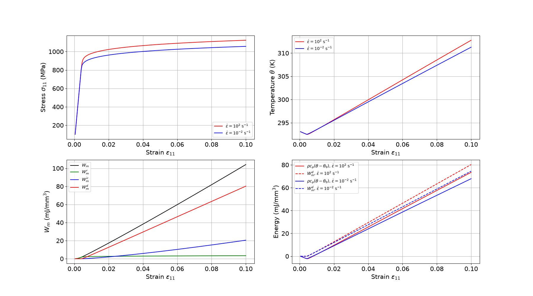
# The same 10 % tension is applied over 10 s, 1 s and 1 ms, i.e. at strain rates of
# :math:`10^{-2}`, :math:`10^{-1}` and :math:`10^{2}` s\ :math:`^{-1}`. The first two sit below
# the reference rate :math:`\dot{\varepsilon}_0 = 1` s\ :math:`^{-1}`, where the rate factor is
# clamped at 1, so they coincide; the fast one hardens by the logarithmic factor. Every path is
# read in Python and the case runs in memory.

rate_configs = {
    "slow": {"pathfile": "EPJCK_path_slow.json", "label": r"$\dot{\varepsilon} = 10^{-2}$ s$^{-1}$"},
    "medium": {"pathfile": "EPJCK_path.json", "label": r"$\dot{\varepsilon} = 10^{-1}$ s$^{-1}$"},
    "fast": {"pathfile": "EPJCK_path_fast.json", "label": r"$\dot{\varepsilon} = 10^{2}$ s$^{-1}$"},
}
colors = {"slow": "blue", "medium": "black", "fast": "red"}

results = {}
for key, cfg in rate_configs.items():
    blocks, T_init, _ = sim.solver.load_path_json(os.path.join(path_data, cfg["pathfile"]))
    results[key] = sim.solver.solve(
        blocks,
        umat_name,
        props,
        nstatev,
        T_init=T_init,
        solver_type=solver_type,
        corate=corate_type,
        orientation=(psi_rve, theta_rve, phi_rve),
    )

fig = plt.figure()
ax1 = fig.add_subplot(1, 2, 1)
ax2 = fig.add_subplot(1, 2, 2)

for key, cfg in rate_configs.items():
    res = results[key]
    e11 = res["Strain"][0]
    s11 = res["Stress"][0]
    time = res["Time"]
    Wm_d = res["Wm"][3]
    # the medium path carries a reverse / reload cycle: plot only its first step
    n = len(e11) if key != "medium" else np.argmax(e11) + 1
    ax1.plot(e11[:n], s11[:n], c=colors[key], label=cfg["label"])
    ax2.plot(time[:n] / time[n - 1], Wm_d[:n], c=colors[key], label=cfg["label"])

ax1.set_xlabel(r"Strain $\varepsilon_{11}$", size=15)
ax1.set_ylabel(r"Stress $\sigma_{11}$ (MPa)", size=15)
ax1.set_title("Strain rate sensitivity (Johnson-Cook, AISI 4340)", size=15)
ax1.grid(True)
ax1.legend(loc="best", fontsize=12)
ax1.tick_params(axis="both", which="major", labelsize=15)

ax2.set_xlabel("normalized time $t / t_{\\textrm{end}}$", size=15)
ax2.set_ylabel(r"Dissipated work $W_m^d$ (mJ/mm$^3$)", size=15)
ax2.set_title("Dissipated work", size=15)
ax2.grid(True)
ax2.legend(loc="best", fontsize=12)
ax2.tick_params(axis="both", which="major", labelsize=15)

plt.tight_layout()
plt.show()

# ###################################################################################
# Reverse loading at the reference rate
# --------------------------------------
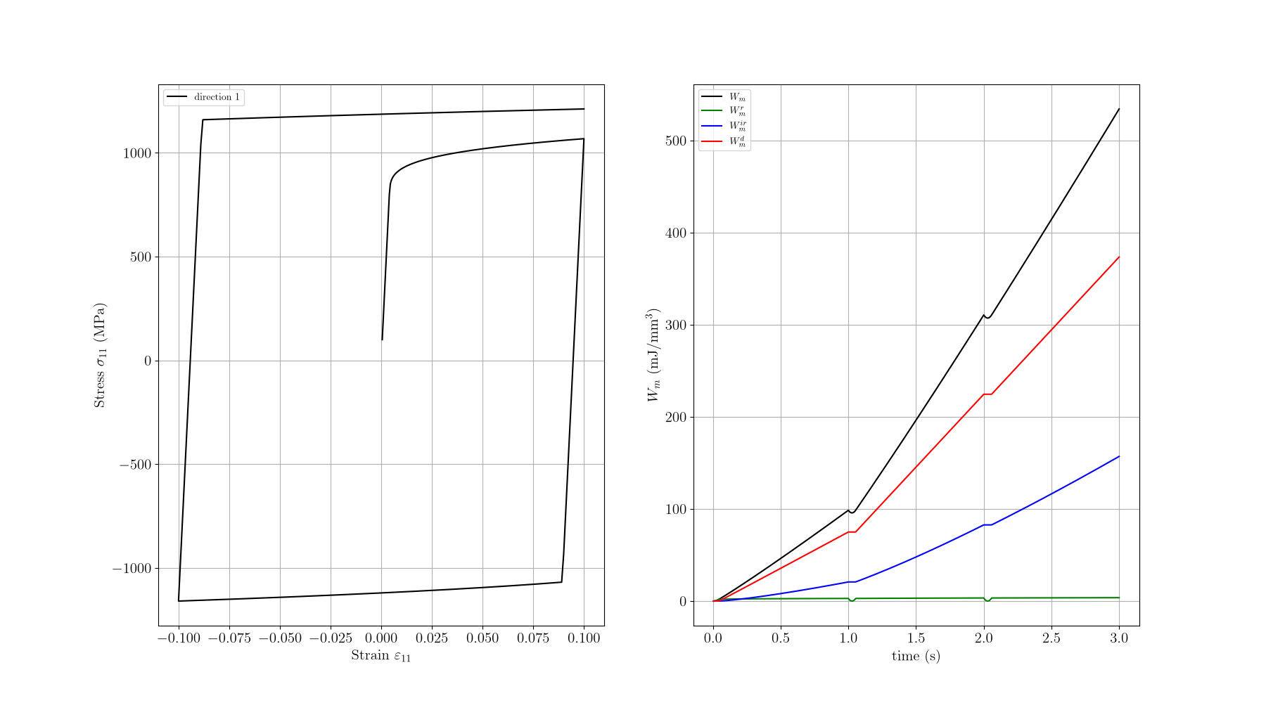
# The medium-rate path continues with a compression to -10 % and a reload to +10 %. The
# hardening is isotropic, so the flow stress keeps growing with :math:`p` on each reversal.

res = results["medium"]
e11 = res["Strain"][0]
s11 = res["Stress"][0]
time = res["Time"]
Wm, Wm_r, Wm_ir, Wm_d = res["Wm"]
p = res["Statev"][1]

fig = plt.figure()
ax = fig.add_subplot(1, 2, 1)
plt.grid(True)
plt.tick_params(axis="both", which="major", labelsize=15)
plt.xlabel(r"Strain $\varepsilon_{11}$", size=15)
plt.ylabel(r"Stress $\sigma_{11}$ (MPa)", size=15)
plt.plot(e11, s11, c="black", label="direction 1")
plt.legend(loc=2)

ax = fig.add_subplot(1, 2, 2)
plt.grid(True)
plt.tick_params(axis="both", which="major", labelsize=15)
plt.xlabel("time (s)", size=15)
plt.ylabel(r"$W_m$ (mJ/mm$^3$)", size=15)
plt.plot(time, Wm, c="black", label=r"$W_m$")
plt.plot(time, Wm_r, c="green", label=r"$W_m^r$")
plt.plot(time, Wm_ir, c="blue", label=r"$W_m^{ir}$")
plt.plot(time, Wm_d, c="red", label=r"$W_m^d$")
plt.legend(loc=2)

plt.show()